Clustering (K-means, Gaussian Mixture Model (GMM) and Expectation Maximization (EM) Algorithm)
12 Jul 2022< 목차 >
- Clustering
- Gaussian Mixture Model (GMM)
- (E)xpectation and (M)aximization
- Kmeans Algorithm
- From MLE to EM to VAE
- References
Clustering
Clustering 을 한다는 뭘까요? 아래의 예시를 봅시다.
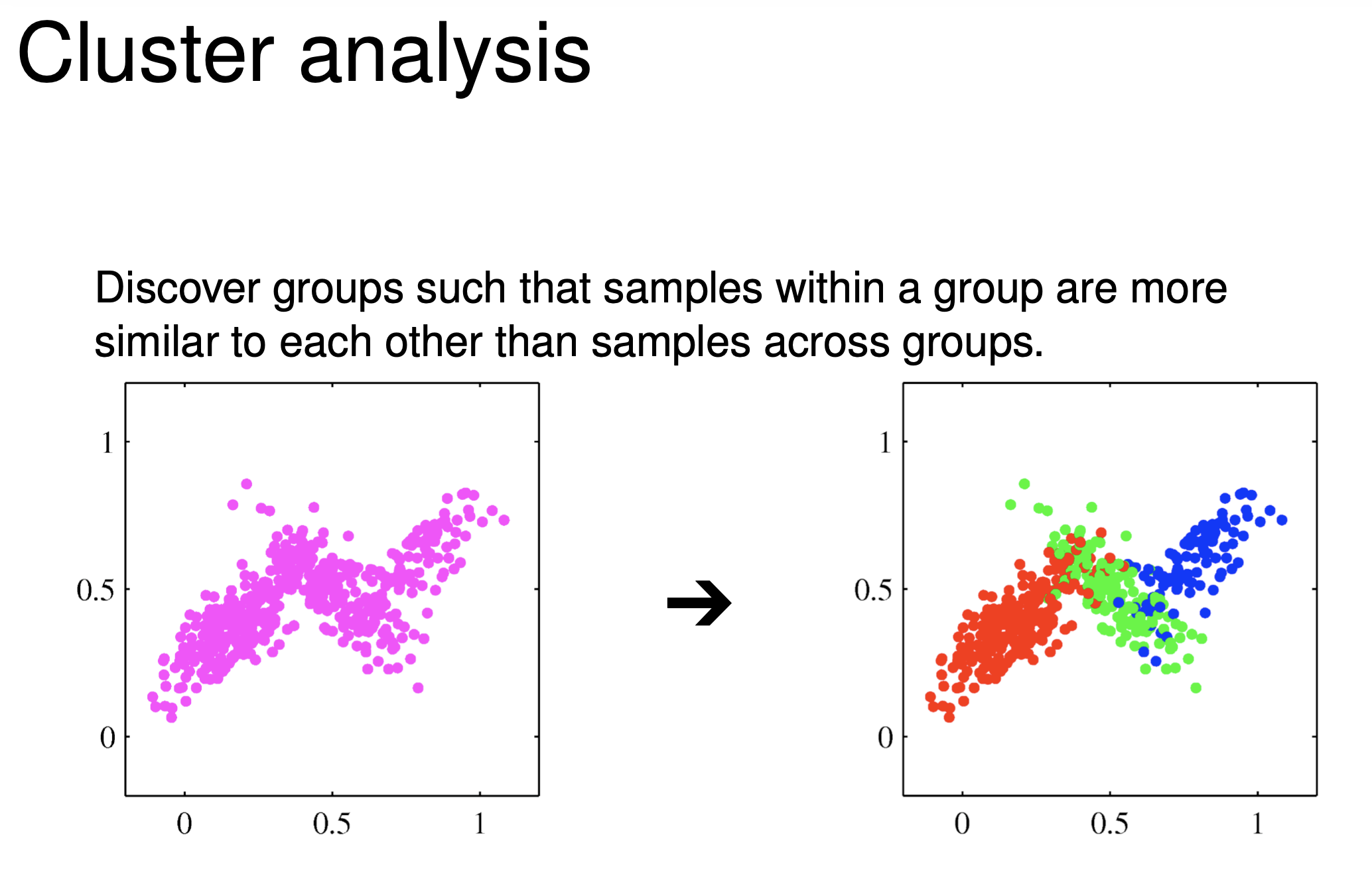 Fig.
Fig.
Clustering 을 한다는 것은 우리가 가지고 있는 dataset 의 data point (sample) 들이 어느 group 에서 샘플링 된 건지 모르지만 이를 의미 있게 여러 group 으로 나눠주는 (또는 모아주는) 것을 말합니다.
즉 데이터 \(x_1\) 은 \(y_1 \in \text{"cat"}\) 이라는 class label 이 존재하지 않지만 잠재적으로 이게 존재한다고 보고 나누겠다는 것으로, 다시 말해 Unsupervised Learning 을 한다는 거죠.
Clustering 을 사용한 Application 으로는 Image Segmentation 이나
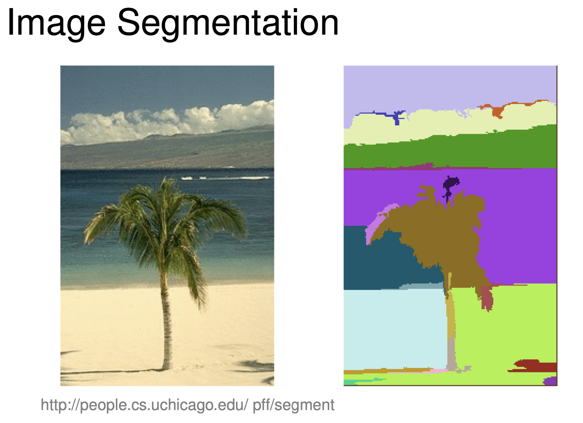 Fig. Image Segmentation using Clustering
Vector Quatization 등이 있다고 합니다.
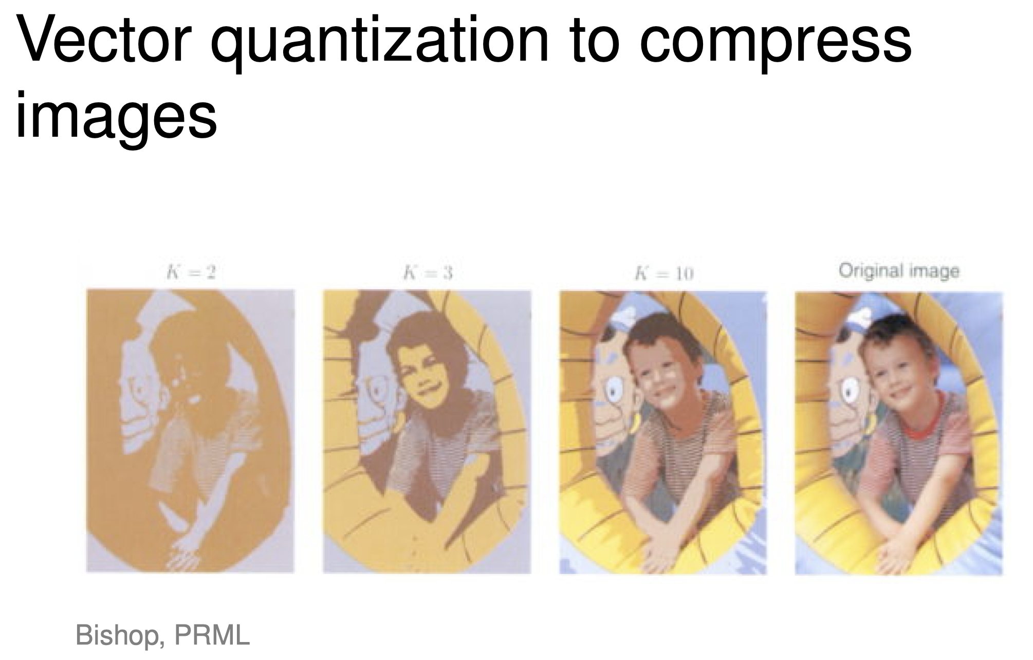 Fig. Vector Quantization using Clustering
그렇다면 Clustering 을 하기 위해서 어떤 게 필요할까요?
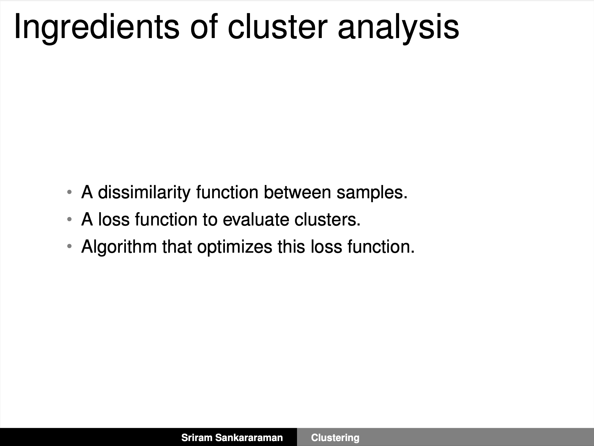 Fig. Source from Sriram Sankararaman’s Slide
위의 슬라이드처럼 세 가지 요소만 있으면 되는데요,
- data point 간 similarity 를 잴 수 있는
dissimilarity function - clustering 이 잘 됐는지를 판단해 줄
objective function (loss function) - objective function 을 최적화 할 algorithm
입니다.
여기서 dissimilarity function 으로는 Euclidean Distance 같은 것을 사용할 수 있고, objective function 을 최적화 할 알고리즘으로는 보통 EM algorithm 을 사용하며, 대표적인 Clustering 알고리즘으로는 K-means나 Gaussian Mixture Model (GMM)이 있습니다.
K-means and Gaussian Mixture Model (GMM) Algorithm
그렇다면 Clustering 을 할 때 K-means 와 GMM 중 어떤 걸 써야 할까요?
둘의 가장 큰 차이 중 하나는 Covariance 를 모델링 할 수 있느냐 없느냐 인데요, GMM 은 Cluster 의 center (mean) 과 그 Cluster 가 얼마나 퍼져있는지 (variance) 모두 learnable 하기 때문에 variance 를 모델링 할 수 있으나 K-means 는 그렇지 않습니다.
다시 말해 K-means 로 Clustering을 하면 그 군집은 둥글게 (공평하게 ?) 모델링 될 수 밖에 없는거죠.
이 말은 아래의 그림처럼 clustering 되어야 할 데이터 샘플들이
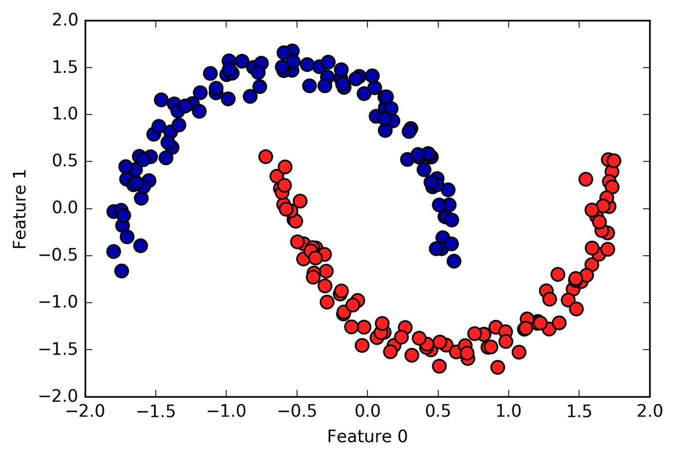 Fig. Limitation of Kmeans. Source from link
이렇게 밖에 군집되지 않는다는 겁니다.
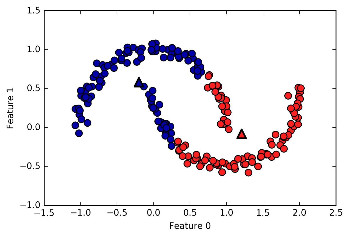 Fig. Limitation of Kmeans. Source from link
(추가 비교)
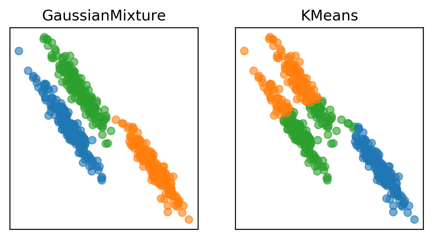 Fig. Comparison between GMM and Kmeans 1. Source from link
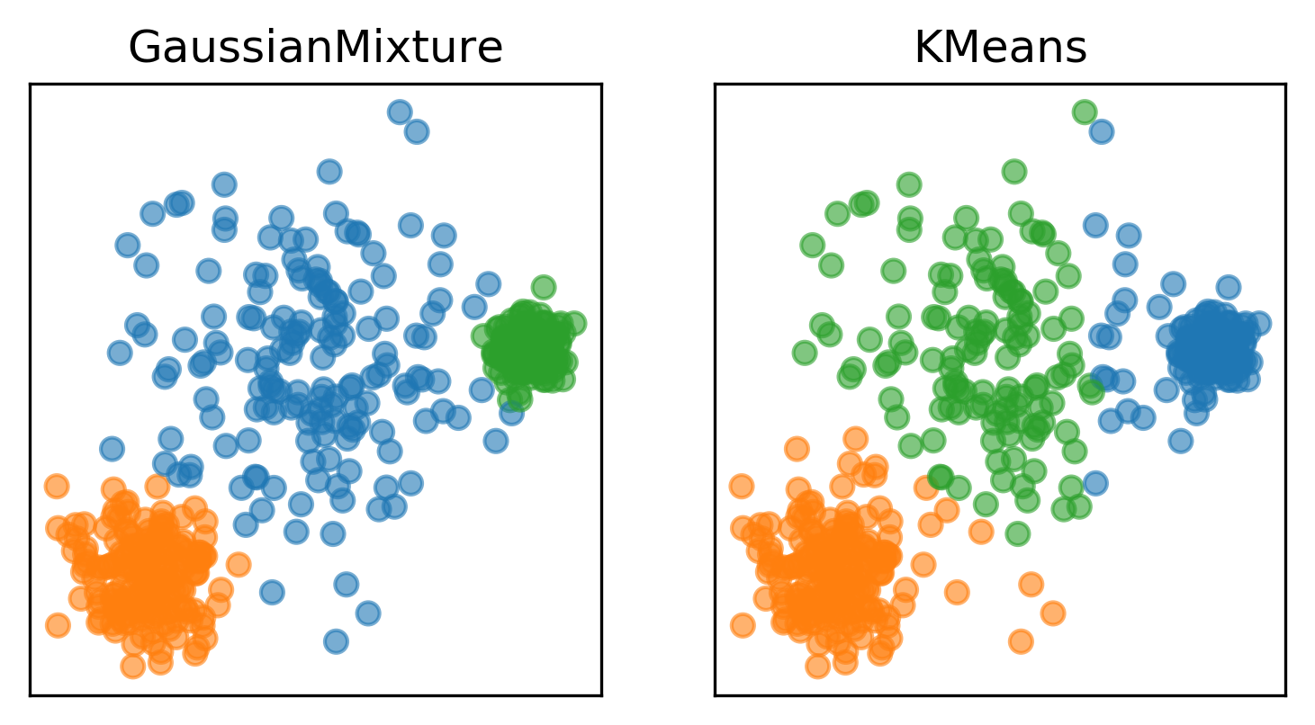 Fig. Comparison between GMM and Kmeans 2. Source from link
나중에 수식적으로도 비교해 보겠지만 K-means 는 GMM 의 hard case 라고 볼 수 있습니다.
(참고 : link)
물론 모든 알고리즘이 일장일단이 있듯 GMM이 더 복잡한 Clustering 을 잘한는 대신 학습하기 어렵다는 등의 단점이 있다고 하니 Clustering 할 일이 있다면 Kmeans 와 GMM 둘 다 고려해보는게 좋겠죠?
아무튼 둘 중에 GMM이 좀 더 general 한 것 같으니 이것부터 살펴보도록 합시다.
Gaussian Mixture Model (GMM)
Models with hidden variables
대부분의 머신러닝/딥러닝 알고리즘은 Maximum likelihood Estimation (MLE) 을 사용해서 최적의 파라메터를 구하죠.
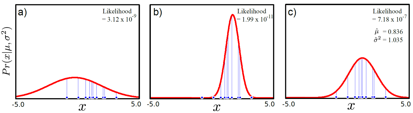 Fig. simple MLE
위의 그림처럼 찾고자 하는 likelihood가 가우시안 분포일 경우 우리가 단지 원하는 것은 likelihood를 최대화 하는 파라메터(mean, variance)를 찾는 거였죠.
GMM 도 마찬가지입니다, target distribution 을 설정하고 이를 최대화 하는 방식으로 학습되죠.
하지만 우리가 추정하고자하는 분포가 한 개의 가우시안 분포보다 더 복잡하다면 어떡할까요? 예를 들어 봉우리가 여러개인(multimodal)인 경우는요?
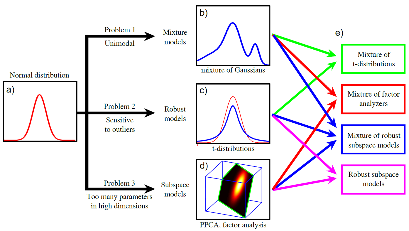 Fig. Problem 1의 mixture model 같은 경우 봉우리가 여러개인 (multimodal) 가우시안 분포이다.
이럴 경우 우리는 찾고자 하는 likelihood p(x) 가 가우시안 분포 두 개, 세 개가 합쳐진 분포라고 생각하고 mean, variance를 세개씩 구해야 하나요? (물론 그럴수도 있겠지만)
이런 경우 분포에 대해서 우리가 알 수 없는 데이터에 내재되어 있는 어떤 숨겨진 변수 (hidden variable) (혹은 잠재 변수 (latent variable이라고 부름)가 있을거라고 생각하고 이를 최대화 하는 방법을 사용할 수 있습니다.
이처럼 GMM 은 우리가 모델링 하고자 하는 target distribution 을 정할 때 하나의 봉우리를 갖는 단봉 (uni-mode) gaussian 분포가 아니라 이런 gaussian 여러 개를 weighted sum 하는 식이지만 얼마만큼의 weight 를 곱해줄지는 모르는 상황이라고 생각할 수 있습니다.
이를 시각화 해보면 아래와 같은데요,
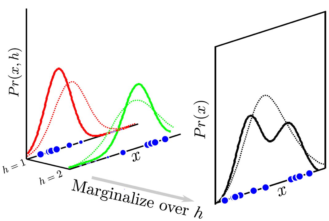 Fig. h를 도입해서 생각하면 봉우리 (mode)가 여러개인 분포처럼 복잡한 분포를 모델링할 수 있다.
원래 분포가 \(Pr(x)\) 였는데 잠재 변수 \(h\)가 껴서 \(Pr(x) = \int Pr(x,h) dh\)가 됐습니다.
말씀드린 것 처럼 h 라는 것은 우리가 가지고 있는 데이터에는 없는 내용입니다. 하지만 이런것이 데이터 내에 내재되어 있다고 생각한거죠.
이 부분이 핵심인데요, 어떤 데이터 100개를 모델링 하는데 있어서 사실 60개는 A class 에서 40개는 B class 에서 샘플링 됐으나 우리는 이 정보를 모르고 있을 때 데이터에는 없는 정보지만 h=1, h=2 라는 fake label 이 존재하고 (h 는 continuos 할 수 있습니다만 지금은 discrete, 특히 binary 인 상황입니다) 잘 학습하기만 한다면 어떤 test sample 이 들어왔을 때 h=1 일 확률이 70% 다 (자동으로 h=2 는 30%) 를 뱉게 되고 그 test sample 은 h=1, 즉 A class 로 분류되는 겁니다.
 Fig. 데이터가 샘플링 된 실제의 다봉 분포에 fitting 되는 과정. Source From link
이 결합 분포는 h 에 대해 적분을 하면 \(Pr(x) = \int Pr(x,h) dh\) 원래의 \(Pr(x)\) 가 되므로 걱정하지 않아도 됩니다. (이 적분식을 최대화 하면 되니까요)
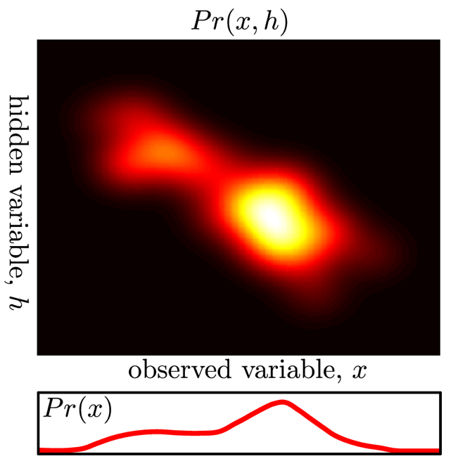 Fig. h가 껴서 Pr(x,h)가 됐다.
그렇다면 어떻게 GMM 을 학습해야 할까요?
여기에 뉴럴 네트워크의 파라메터 \(\theta\) 가 있다고 생각해 봅시다.
\[Pr(x|\theta) = \int Pr(x,h|\theta) dh\]데이터 포인트가 당연히 여러개 이겠고 iid 라는 가정을 하고, numerical stability 를 위해서 logarithm 을 취해주면 \(\sum\) 과 \(log\) 가 붙겠죠?
\[\hat{\theta} = \arg \max_{\theta} [ \sum_{i=1}^{I} log [\int Pr(x_i,h_i|\theta) dh_i] ]\]이제 어떻게 하면 위의 파라메터를 최대화 할 수 있을까요?
(E)xpectation and (M)aximization
Lower Bound
GMM 같은 잠재 변수 모델의 log likelihood 를 최대화 하는 방법은 바로 (E)xpectation and (M)aximization Algorithm 을 사용하는 겁니다.
이는 log likelihood에 대한 lower bound를 정의하고 반복해서 그 bound를 증가시키면 결국에 likelihood 를 최대화 하는 것과 같은 효과라는 내용인데요, 그럼 lower bound 를 한 번 구해봅시다.
먼저 현재 수식에 위아래로 \(\frac{q(h)}{q(h)}\) 를 곱해봅시다. 당연히 이 값은 1이기 때문에 곱해줘도 수식적으로 문제가 없고, Jansen’s inequality 를 사용하면 아래와 같은 부등식을 얻을 수 있습니다.
\[\begin{aligned} & B[\{ q_i(h_i) \}, \theta] = \sum_{i=1}^{I} \int q_i(h_i) log[\frac{Pr(x,h_i|\theta)}{q_i(h_i)}]dh_{1...I} & \\ & \leq [ \sum_{i=1}^{I} log [\int Pr(x_i,h|\theta) dh_i] ] & \\ \end{aligned}\]즉 좌변을 최대화 하는 것이 우변의 원래의 log likelihood 를 최대화 하는 것이죠.
다시 말해 왼쪽의 bound B 를 높히면 오른쪽에 있는 항은 덩달아 올라갈 수 밖에 없는 겁니다.
E-Step
우리가 사용할 bound 를 높히는 방법은 Expectation (E) Step과 Maximization (M) Step 두 process 를 반복적으로 (iteratively) 번갈아가면서 수행하는 EM Algorithm입니다.
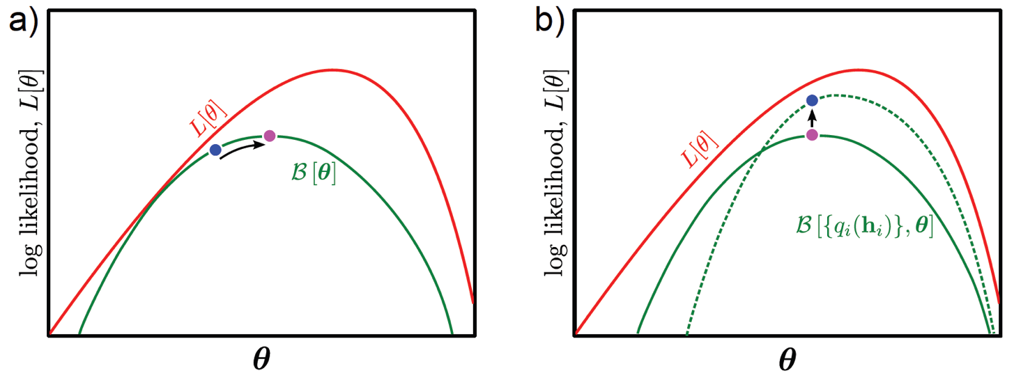 Fig. E Step (a) 한 번, M Step (b) 한 번 이 한 세트
여기서 E Step은 주어진 파라메터의 초기값에 대해서 likelihood와 최대한 근사한 likelihood를 얻어내는 것으로 즉 \(q(h_i)\) 에 대해서 bound 를 최대화 하는 것이고,
M Step은 이 \(\theta\) 에 대해 likelihood를 최대화 하는 방향으로 파라메터를 업데이트 하는 겁니다.
E Step 을 먼저 볼까요? 분포 \(q_i(h_i)\)에 대해서 bound를 최대화 하는 것으로 수식으로 나타내면 아래와 같습니다.
\[\hat{q_i}(h_i) = Pr(h_i|x_i,\theta^{[t]}) = \frac{Pr(x_i|h_i,\theta^{[t]}) Pr(h_i|\theta^{[t]})}{Pr(x_i)}\]M-Step
M Step은 분포 \(\theta\)에 대해서 bound를 최대화 하는 것으로 수식으로 나타내면 아래와 같습니다.
\[\hat{\theta}^{[t+1]} = \arg \max_{\theta} [ \sum_{i=1}^{I} \int \hat{q_i}(h_i) log [Pr(x_i,h_i|\theta)] dh_i ]\]이 두 가지 step을 iterative하게 그림으로 나타내면 아래와 같습니다.
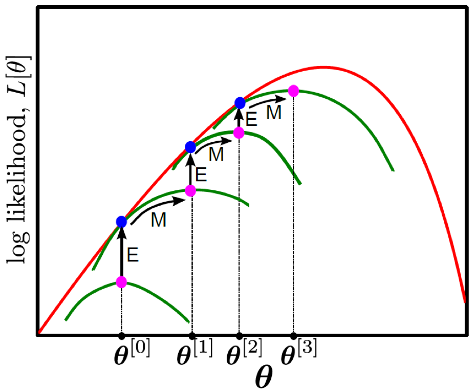 Fig.
Fig.
GMM Example
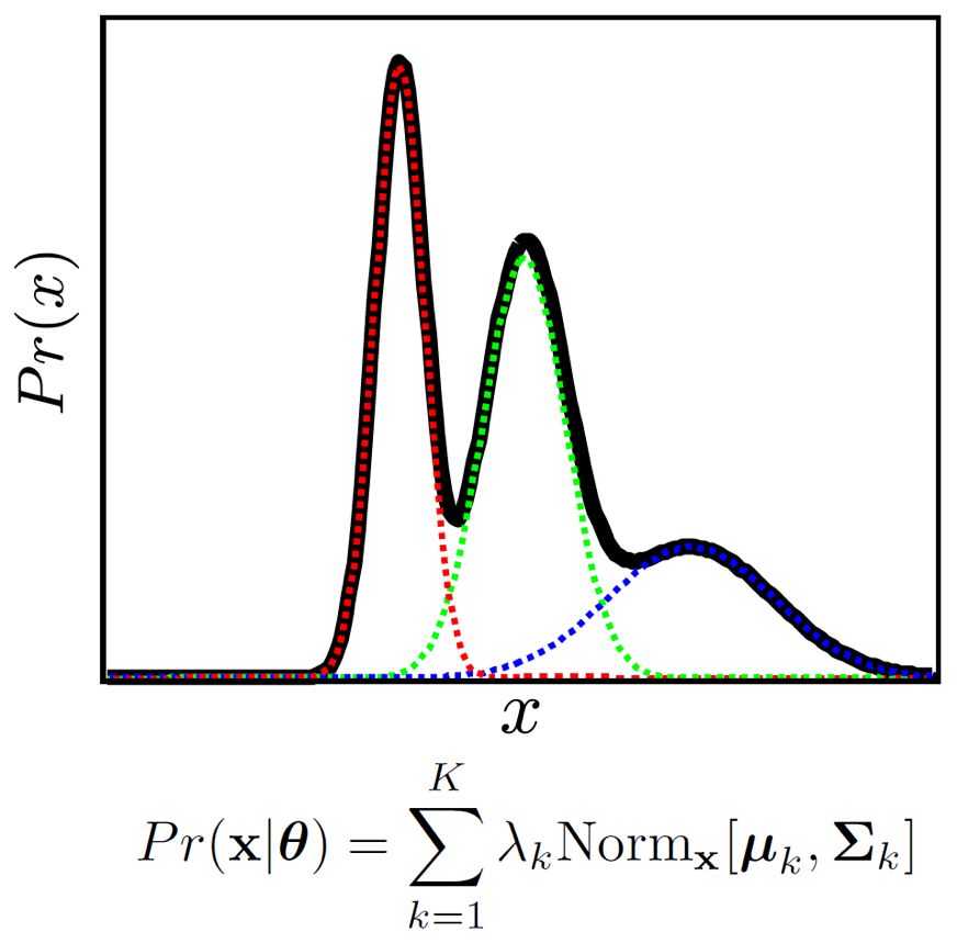 Fig.
Fig.
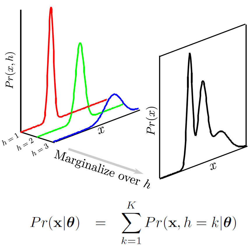 Fig.
Fig.
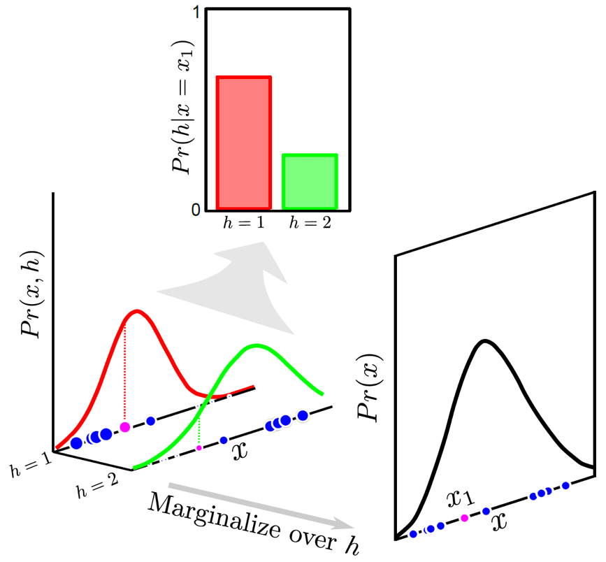 Fig.
Fig.
Fig.
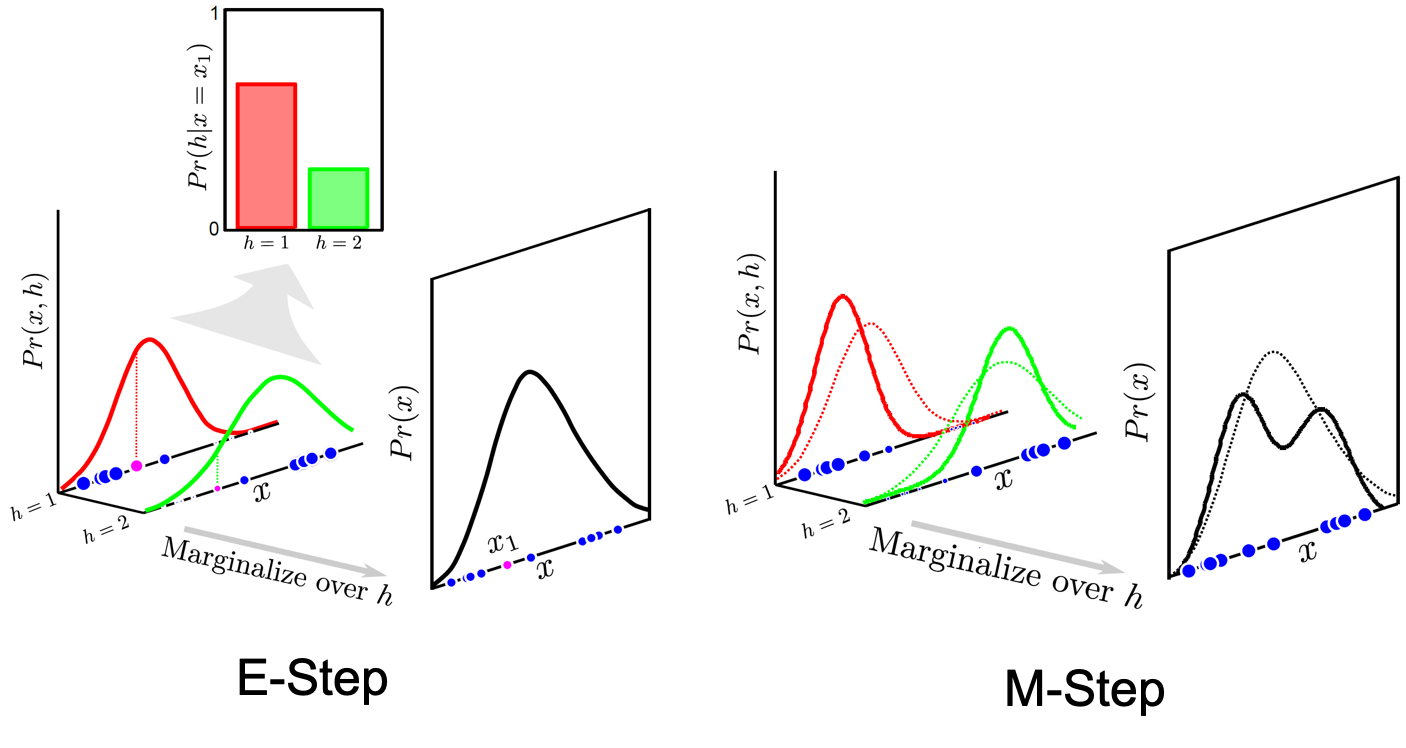 Fig.
Fig.
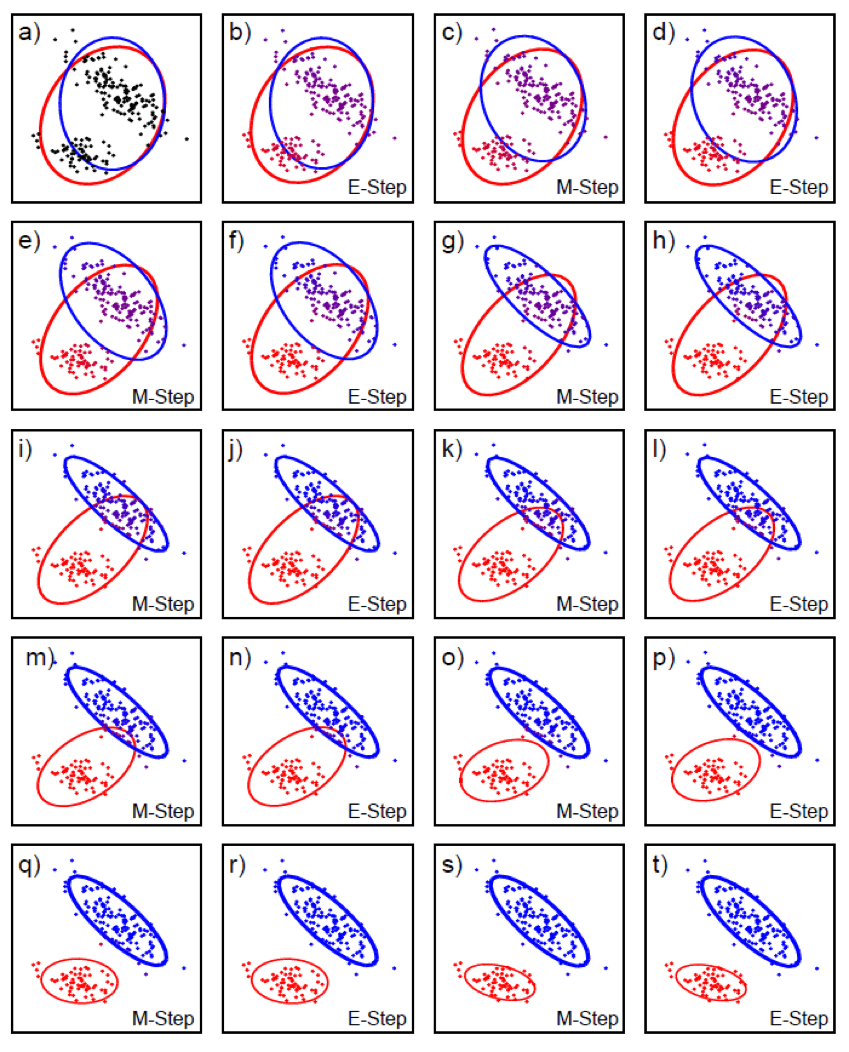 Fig.
Fig.
asd
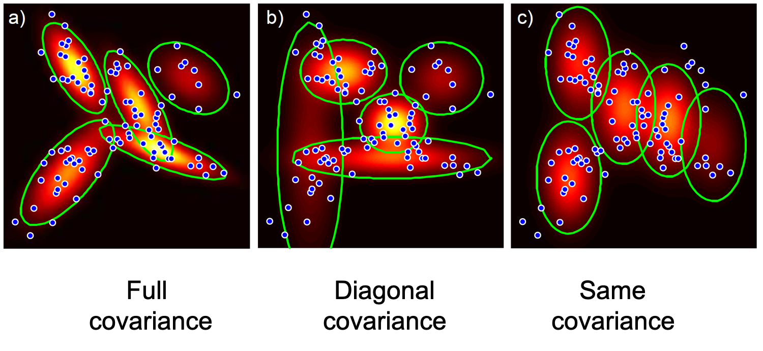 Fig.
Fig.
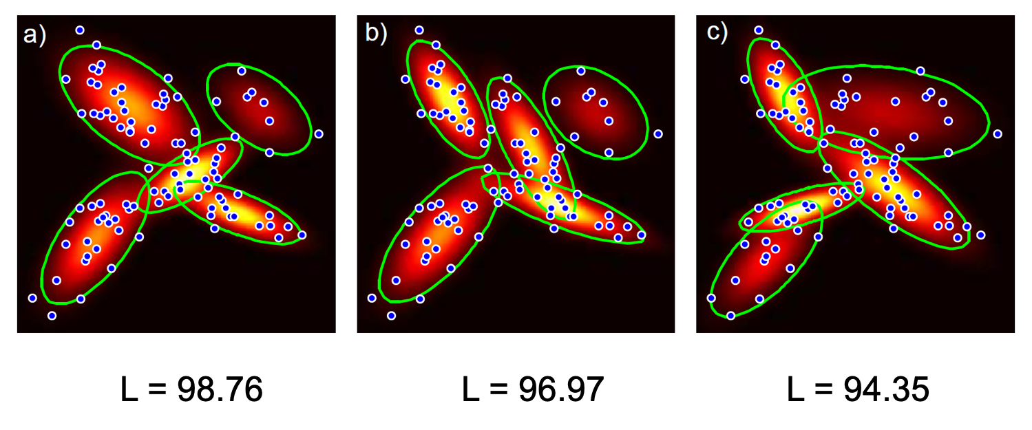 Fig.
Fig.
Kmeans Algorithm
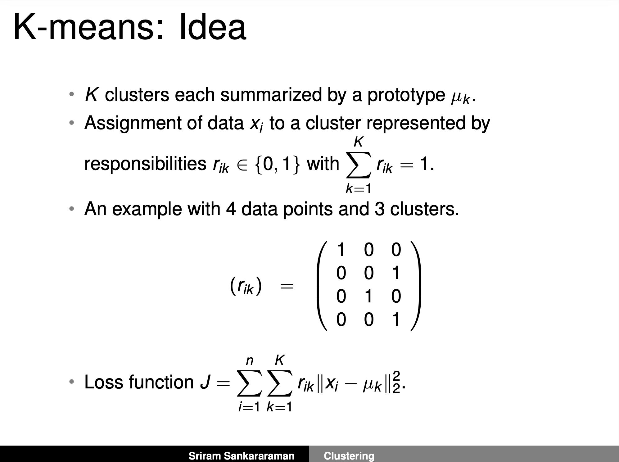 Fig.
Fig.
 Fig.
Fig.
EM Algorithm again
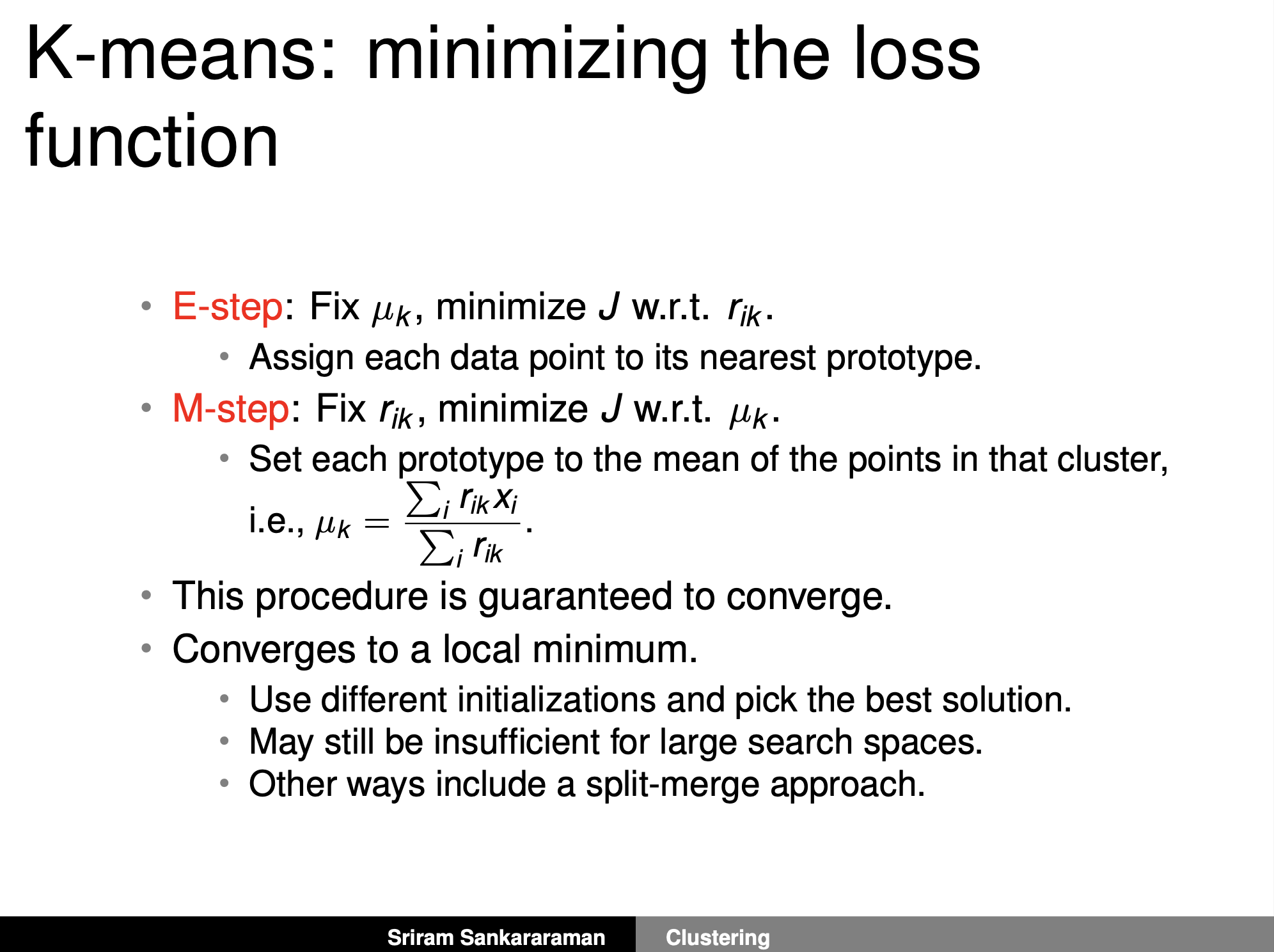 Fig.
Fig.
 Fig.
Fig.
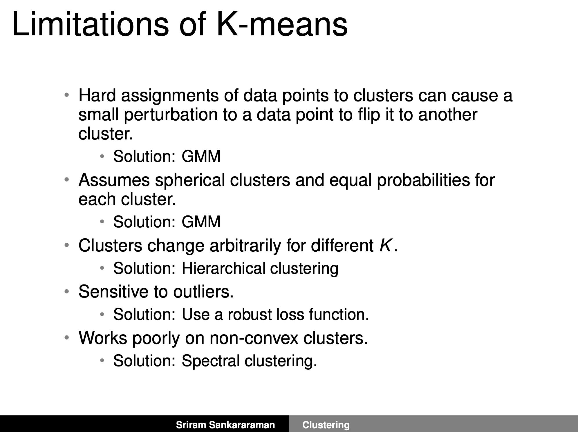 Fig.
Fig.
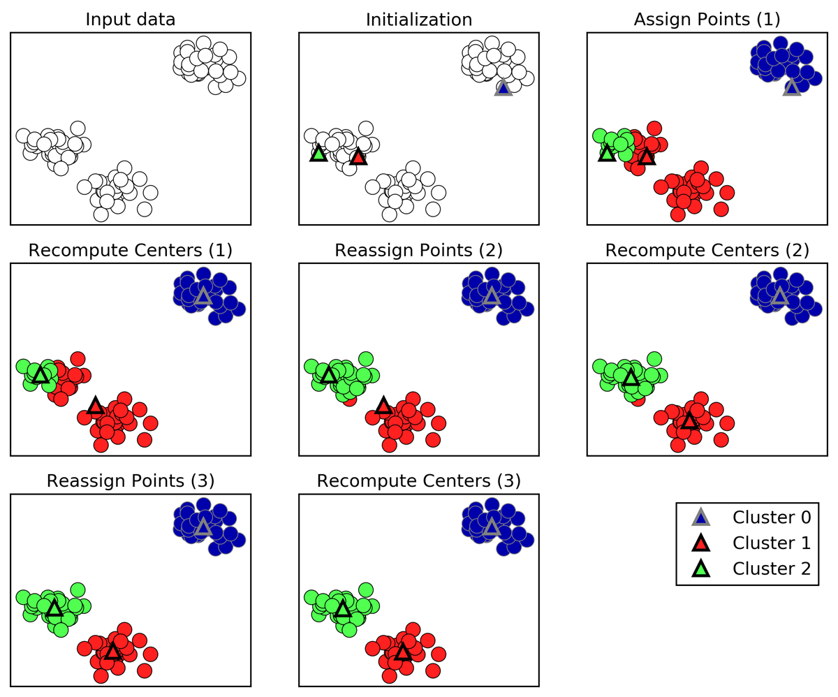 Fig.
Fig.
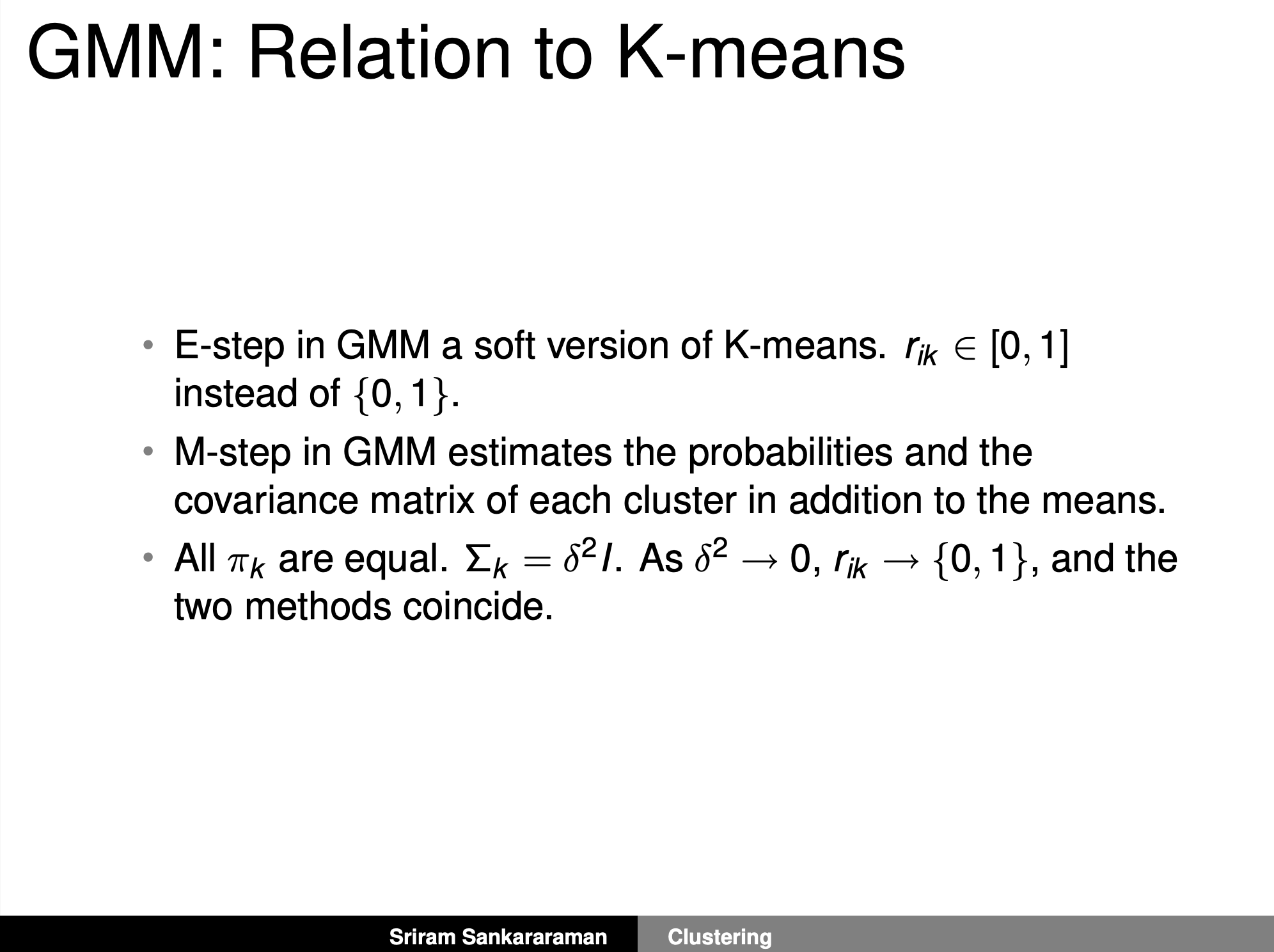 Fig.
Fig.
From MLE to EM to VAE
 Fig.
Fig.
 Fig.
Fig.
References
- Books
- Others
- Unsupervised Learning cheatsheet by Afshine Amidi and Shervine Amidi
- The road from MLE to EM to VAE: A brief tutorial
- What’s the relationship between Variational Autoencoders and the Expectation Maximization Algorithm?
- Auto-Encoding Variational Bayes
- Slide from Sriram Sankararaman
- Clustering and Mixture Models from Andreas C. Müller