Pytorch Implementation of Variational AutoEncoders (VAEs)
22 May 2022< 목차 >
- AutoEncoder (AE)
- Variational AutoEncoder (VAE)
- Vector Quantized Variational AutoEncoder (VQ-VAE)
- References
이번 post 에서는 Variational AutoEncoder (VAE) 모델들을 직접 학습해보려고 합니다.
Alexander Van de Kleut의 post를 base로 삼았습니다.
VAE 에 관한 이론적인 내용은 저의 블로그 내 다른 post 를 참고하시면 좋을 것 같습니다.
AutoEncoder (AE)
VAE를 구현하기 전에 유사한 구조체인 Auto Encoder (AE)를 먼저 학습해보려고 합니다.
(물론 구조가 비슷하지만 VAE는 생성모델, 그리고 잠재변수 모델이라는 점을 잊으시면 안됩니다.)
AE 는 다음과 같이 생겼는데요,
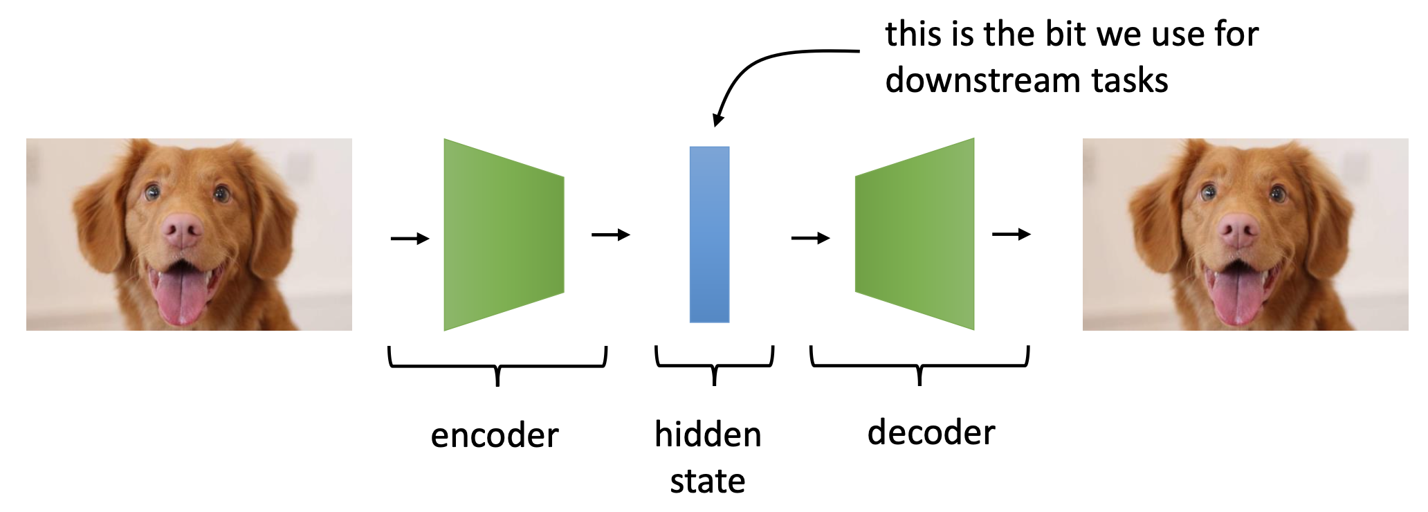 Fig. Encoder 와 Decoder 로 이루어진 아주 간단한 AutoEncoder 모델
다들 아시다시피 input 정보를 압축하는 Encoder와 이를 복원하는 Decoder 가 있으며, 목적은 input 을 잘 나타내는 feature (representation) 을 encoder가 학습하는 것입니다. (이걸 나중에 task에 맞게 finetuning 하는 방법으로 BERT 등의 원조라고 할 수 있죠.)
Encoder와 Decoder를 아래처럼 간단하게 구성해줍니다.
class Encoder(nn.Module):
    def __init__(self, image_size, num_channel, latent_dims):
        super(Encoder, self).__init__()
        self.linear1 = nn.Linear(image_size**2 * num_channel, 512)
        self.linear2 = nn.Linear(512, latent_dims)

    def forward(self, x):
        x = torch.flatten(x, start_dim=1)
        x = F.relu(self.linear1(x))
        return self.linear2(x)
class Decoder(nn.Module):
    def __init__(self, image_size, num_channel, latent_dims):
        super(Decoder, self).__init__()
        self.linear1 = nn.Linear(latent_dims, 512)
        self.linear2 = nn.Linear(512, image_size**2 * num_channel)
        self.image_size = image_size
        self.num_channel = num_channel

    def forward(self, z):
        z = F.relu(self.linear1(z))
        z = torch.sigmoid(self.linear2(z))
        return z.reshape((-1, self.num_channel, self.image_size, self.image_size))
왜 Decoder의 최종 출력값이 0~1로 매핑되느냐? (sigmoid를 왜 쓰느냐?), 그 이유는 우리가 사용할 데이터셋이 MNIST 인데 이 데이터는 흑백 이미지 데이터로 각 픽셀값이 0~1 로 이루어져 있기 때문입니다.
이제 이 인코더가 뱉은걸 디코더가 받도록 구성해주면 끝입니다.
class Autoencoder(nn.Module):
    def __init__(self, image_size, num_channel, latent_dims):
        super(Autoencoder, self).__init__()
        self.encoder = Encoder(image_size, num_channel, latent_dims)
        self.decoder = Decoder(image_size, num_channel, latent_dims)

    def forward(self, x):
        z = self.encoder(x)
        return self.decoder(z)
간단하게 argparser로 몇 가지 인자를 정의해주고요,
parser = argparse.ArgumentParser()
parser.add_argument('--dataset_dir_path', type=str, default='./data')
parser.add_argument('--batch_size', type=int, default=256)
parser.add_argument('--num_epoch', type=int, default=25)

parser.add_argument('--lr', type=float, default=0.001)
parser.add_argument('--lr_step', type=float, default=1.0)
parser.add_argument('--latent_dims', type=int, default=2)

parser.add_argument('--log_interval', type=int, default=50)
parser.add_argument('--plot', action='store_true')

args = parser.parse_args()
아래처럼 torchvision library의 데이터셋을 사용해서 data loader를 만듭니다.
dataset = torchvision.datasets.MNIST(args.dataset_dir_path,
            train=True,
            transform=torchvision.transforms.ToTensor(),
            download=True)
dataset_test = torchvision.datasets.MNIST(args.dataset_dir_path,
            train=False,
            transform=torchvision.transforms.ToTensor(),
            download=True)
image_size = 28
num_channel = 1

data_loader = torch.utils.data.DataLoader(dataset, batch_size=args.batch_size, shuffle=True,num_workers=4)
data_loader_test = torch.utils.data.DataLoader(dataset_test, batch_size=args.batch_size, shuffle=False,num_workers=4)
학습을 하려면 아까 만든 Autoencoder class를 모델로 선언해주고 optimizer 등을 정의해줘야겠죠?
model = Autoencoder(image_size, num_channel, args.latent_dims).to(device)
optimizer = torch.optim.AdamW(model.parameters(), lr=args.lr)
lr_scheduler = torch.optim.lr_scheduler.StepLR(optimizer, step_size=int(args.num_epoch*args.lr_step), gamma=0.333)
이제 data loader, model 그리고 optimizer 를 사용해서 training loop 를 돌리면 됩니다.
    for epoch in range(args.num_epoch):
        train_num_batches = len(data_loader)
        test_num_batches = len(data_loader_test)

        model.train()
        lr = lr_scheduler.get_last_lr()[0]
        for i, (x,y) in enumerate(data_loader):

            x = x.to(device)
            pred = model(x)
            loss = F.mse_loss(pred, x, reduction='sum')
            optimizer.zero_grad()
            loss.backward()
            optimizer.step()

            if i % args.log_interval == 0 and i > 0:
                print(f'| epoch {epoch:3d} | '
                    f'{i:5d}/{train_num_batches:5d} batches | '
                    f'lr {lr:02.4f} | '
                    f'loss {loss:5.3f}')

        model.eval()
        val_loss = 0.0
        for i, (x,y) in enumerate(data_loader_test):
            x = x.to(device)
            with torch.no_grad():
                pred = model(x)
                loss = F.mse_loss(pred, x, reduction='sum')
                val_loss += loss.item()

        print(f'| epoch {epoch:3d} | lr {lr:02.4f} | total validation loss {val_loss/test_num_batches:5.3f}')

        lr_scheduler.step()
아주 간단하죠.
    pred = model(x)
    loss = F.mse_loss(pred, x, reduction='sum')
특히 단순하게 이미지 픽셀을 원본과 비교하면서 복원하는게 전부이기 때문에 loss는 mse loss를 쓴 걸 알 수 있습니다.
(하지만 저의 post에서도 설명했듯 흑백 이미지는 픽셀이 0이냐 1이냐로 나눌 수도 있기 때문에 Binary Cross Entropy (BCE)를 사용해서 학습해도 됩니다.)
마지막으로 학습 결과로 Encoder가 어떻게 mnist 이미지를 학습했는지 보도록 하겠습니다.
    if args.plot:
        save_dir_path = os.path.join(os.getcwd(),'assets')
        if not os.path.isdir(save_dir_path) : os.mkdir(save_dir_path)
        plot_latent(model, data_loader_test, save_dir_path)
        plot_reconstructed(model, image_size, num_channel, save_dir_path, r0=(-10, 10), r1=(-10, 10), n=15)
위에서 사용한 plot 함수는 아래처럼 정의됩니다.
def plot_latent(model, data_loader, save_dir_path):
    plt.clf()
    for i, (x, y) in enumerate(data_loader):
        z = model.encoder(x.to(device))
        z = z.to('cpu').detach().numpy()
        plt.scatter(z[:, 0], z[:, 1], c=y, cmap='tab10')
    plt.colorbar()
    file_path = os.path.join(save_dir_path,'latent_space.png')
    if os.path.exists(file_path) : os.remove(file_path)
    plt.savefig(file_path)
def plot_reconstructed(model, image_size, num_channel, save_dir_path, r0=(-3, 3), r1=(-3, 3), n=15):
    plt.clf()
    w = image_size
    img = np.zeros((n*w, n*w, num_channel))
    for i, y in enumerate(np.linspace(*r1, n)):
        for j, x in enumerate(np.linspace(*r0, n)):
            z = torch.Tensor([[x, y]]).to(device)
            x_hat = model.decoder(z)
            x_hat = x_hat.reshape(num_channel, image_size, image_size)
            recon_img = x_hat.permute(1, 2, 0).to('cpu').detach().numpy()
            img[(n-1-i)*w:(n-1-i+1)*w, j*w:(j+1)*w, :] = recon_img
    plt.imshow(img, extent=[*r0, *r1])
    file_path = os.path.join(save_dir_path,'reconstruct_images.png')
    if os.path.exists(file_path) : os.remove(file_path)
    plt.savefig(file_path)
저장된 plot 이미지를 보면 아래와 같은데요,
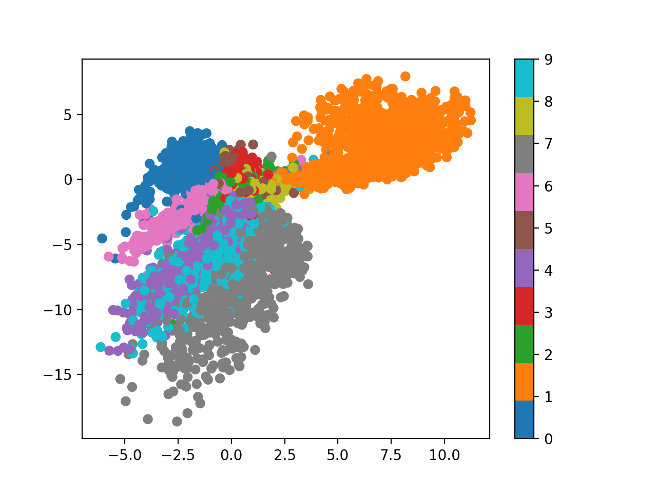 Fig. 2-dim Latent Space from AutoEncoder
첫 번째 이미지는 우리가 AutoEncoder의 hidden dimension, 즉 latent dimension 을 2로 정했기 때문에 이를 2차원 좌표상에 나타낸 겁니다.
잘 보시면 어느정도 같은 숫자를 나타내는 데이터들이 뭉치는걸 볼 수 있지만 딱히 맘에 들지는 않습니다.
여러 이유가 있을 수 있겠죠,
- model 이 너무 간단하다.
- lr, num_epoch 등 하이퍼 파라메터가 적절하지 못했다.
등등..?
그 다음으로는 우리가 2차원 좌표상에 Latent Vector들이 어떻게 매핑됐는지 이해했으니 거기서부터 이미지를 복원해보고 이를 plot해본 건데요,
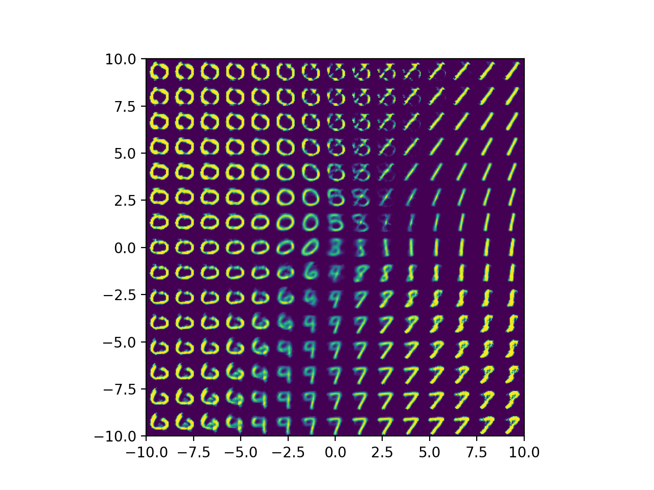 Fig. Decoded Images from 2-dim Latent Space Points
1사분면쪽에서 복원한 이미지들은 대부분 1인걸로 봐서 디코더도 적당히 학습된걸 알 수 있습니다.
Variational AutoEncoder (VAE)
이제 VAE 입니다.
AE와 유사한 구조를 가지고 있지만 몇 가지 다른점이 있는데요,
- Encoder는 Latent Dim 차원의 Vector를 뱉는게 아니라, Latent Dim 차원의
가우시안 분포(다른거여도 되긴 하지만 보통 normal dist) 를 예측한다. 즉 가우시안 분포의 mean 값을 예측함. ELBO Objective를 썼다. (MSE Loss +KL Divergence Loss)- 미분 불가능한 샘플링 연산을 처리하기 위해
Reparameterization Trick을 썼다.
가 주요 차이점 입니다.
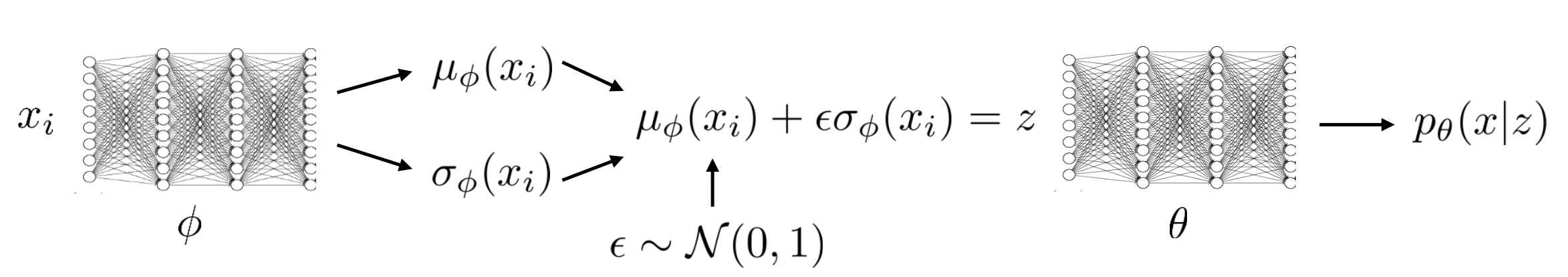 Fig. VAE의 Encoder는 Fixed Vector가 아닌 어떠한 분포를 예측한다.
VAE는 AE랑 구조 자체는 다른게 크게 없으니 구현체도 비슷합니다.
class VariationalAutoencoder(nn.Module):
    def __init__(self, image_size, num_channel, latent_dims):
        super(VariationalAutoencoder, self).__init__()
        self.encoder = Encoder(image_size, num_channel, latent_dims)
        self.decoder = Decoder(image_size, num_channel, latent_dims)

    def forward(self, x):
        z = self.encoder(x)
        return self.decoder(z)
Decoder도 뭐 latent vector z를 받아서 원래 이미지사이즈의 Tensor를 뱉는거니 크게 다른건 없는데요,
class Decoder(nn.Module):
    def __init__(self, image_size, num_channel, latent_dims):
        super(Decoder, self).__init__()
        self.linear1 = nn.Linear(latent_dims, 512)
        self.linear2 = nn.Linear(512, image_size**2 * num_channel)
        self.image_size = image_size
        self.num_channel = num_channel

    def forward(self, z):
        z = F.relu(self.linear1(z))
        z = torch.sigmoid(self.linear2(z))
        return z.reshape((-1, self.num_channel, self.image_size, self.image_size))
문제는 Encoder 입니다.
class Encoder(nn.Module):
    def __init__(self, image_size, num_channel, latent_dims):
        super(Encoder, self).__init__()
        self.linear1 = nn.Linear(image_size**2 * num_channel, 512)
        self.linear_mean = nn.Linear(512, latent_dims) # for mean
        self.linear_variance = nn.Linear(512, latent_dims) # for variance

        self.N = torch.distributions.Normal(0, 1) # zero mean, unit variance gaussian dist
        if device == 'cuda':
            self.N.loc = self.N.loc.cuda() # hack to get sampling on the GPU
            self.N.scale = self.N.scale.cuda()

        self.kld = 0

    def forward(self, x):
        x = torch.flatten(x, start_dim=1)
        x = F.relu(self.linear1(x))

        mu = self.linear_mean(x) # mean
        sigma = torch.exp(self.linear_variance(x)) # variance
        z = mu + sigma * self.N.sample(mu.shape) # sampled with reparm trick

        self.kld = (sigma**2 + mu**2 - torch.log(sigma) - 1/2).sum() # closed-form kl divergence solution

        return z
이전 AE Encoder와 다른게 좀 있는데요, 바로 input을 hidden vector로 매핑하는 linear1 layer 뒤에 mean 과 variance 를 예측하는 linear layer가 각각 2개나 있다는 겁니다.
즉 아래의 그림처럼 하기 위해서 각각을 예측하는 레이어가 두 개 있는거죠.
여기에서 아래 부분이 중요한데요,
        mu = self.linear_mean(x) # mean
        sigma = torch.exp(self.linear_variance(x)) # variance
        z = mu + sigma * self.N.sample(mu.shape) # sampled with reparm trick
VAE에 대해서 다시 생각해봅시다.
- VAE
- What we want : \(p(x) = \int p(y \vert z) p(z) dz\)
- Encoder : \(q_{\phi}(z \vert x_i)\)
- Decoder : \(p_{\theta}(x_i \vert z)\)
ELBO: \(L(p_{\theta}(x_i \vert z), q_{\phi}(z \vert x_i)) = \mathbb{E}_{z \sim q_{\phi}(z \vert x_i)} [log p(x_i \vert z) + log p(z)] + H(q_{\phi}(z \vert x_i))\)
VAE는 ELBO 수식에 보면 이미지를 encoder에 태우면 어떤 분포 (보통 가우시안 분포)가 나오는데 여기에 기대값이 취해져 있습니다. 즉 원래같았으면 그 분포에서 뽑을 수 있는 z vector 는 다 뽑아서 계산을 해야 하는데 이건 불가능하므로 Sampling을 몇 번 하는걸로 대체하는겁니다.
즉 위의 코드에서 보면 가우시안 분포의 mean, variance값을 출력하는 각각의 레이어를 통과한건 알겠는데 여기에서 sigma에 어떤 self.N이라는 zero-mean unit variance 의 가우시안분포에서 뽑은 어떤 값을 곱해주는걸 알 수 있는데, 이게 바로 sampling효과를 내지만 미분을 가능하게 해주는 Reparameterization Trick 입니다.
- VAE
- ELBO : \(L(p_{\theta}(x_i \vert z), q_{\phi}(z \vert x_i)) = \mathbb{E}_{z \sim q_{\phi}(z \vert x_i)} [log p(x_i \vert z) + log p(z)] + H(q_{\phi}(z \vert x_i))\)
- Final Objective : \(\hat{\theta},\hat{\phi} = arg max_{\theta,\phi} ( \sum_{i=1}^{N} [ log p_{\theta} (x_i \vert \mu_{\phi} (x_i) + \epsilon \sigma_{\phi} (x_i) ) - D_{KL} ( q_{\phi} (z \vert x_i ) \parallel p(z) ) ] )\)
위의 수식에서 \(\epsilon\) 이 variance \(\sigma\)와 곱해져서 더해지는 부분이 바로 이 부분입니다.
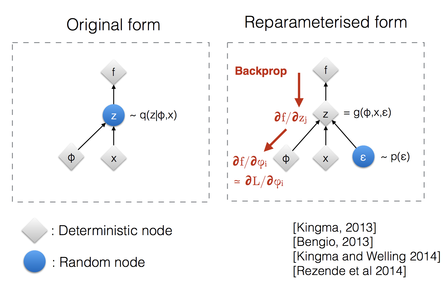 Reparameterization Trick은 Sampling 효과를 내도록 해주지만 미분불가능한 Sampling 연산이 아니므로 end-to-end로 VAE를 학습할 수 있게 해준다.
그리고 코드에서 눈에 띄는 점이 하나 더 있는데요, 바로 뉴럴넷을 forwarding 하면서 self.kld 라는 값을 계산해 낸다는 점입니다.
    def forward(self, x):
        x = torch.flatten(x, start_dim=1)
        x = F.relu(self.linear1(x))

        mu = self.linear_mean(x) # mean
        sigma = torch.exp(self.linear_variance(x)) # variance
        z = mu + sigma * self.N.sample(mu.shape) # sampled with reparm trick

        self.kld = (sigma**2 + mu**2 - torch.log(sigma) - 1/2).sum() # closed-form kl divergence solution

        return z
이 부분은 원래 Objective Function 에 있는 두 항 중 우항에 해당하는 것인데요,
\[\hat{\theta},\hat{\phi} = arg max_{\theta,\phi} ( \sum_{i=1}^{N} [ log p_{\theta} (x_i \vert \mu_{\phi} (x_i) + \epsilon \sigma_{\phi} (x_i) ) - D_{KL} ( q_{\phi} (z \vert x_i ) \parallel p(z) ) ] )\]이건 \(p(z)\) 라는 매우 간단한 가우시안 분포와 Encoder가 뱉은 가우시안 분포 \(q_{\phi}(z \vert x)\) 사이의 KL Divergence (KLD) 이므로, 두 가우시안 분포의 KLD 이기 때문에 closed-form solution이 이미 알려져 있어서 이를 사용한 겁니다.
마지막으로 VAE 학습시에는 아까 봤던 디코더가 z를 받아서 원본을 복원하는 reconstruction loss (AE에서도 봤던 mse loss와 아예 같음) 에 kld loss를 더해주면 끝입니다.
    x = x.to(device)
    pred = model(x)
    recon_loss = loss = F.mse_loss(pred, x, reduction='sum')
    kld_loss = model.encoder.kld
    loss = recon_loss + args.kld_weight * kld_loss
아주 간단하죠?
마찬가지로 plot을 해보자면 아래와 같은 이미지를 얻을 수 있는데요, (마찬가지로 latent vector의 차원은 2차원이고, 같은 encoder, decoder 구조로 25에폭 돌렸습니다.)
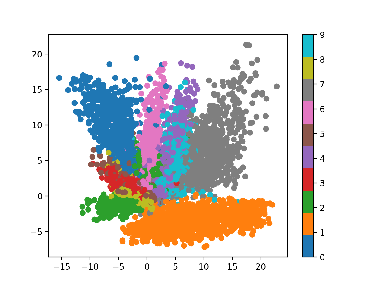 Fig. 2-dim Latent Space from AutoEncoder (VAE)
2차원 분포 상에 좀 더 둥글게, 즉 가우시안 분포 내에 같은 숫자들은 같이 뭉친걸 (semantic clustering) 볼 수 있습니다.
마찬가지로 디코더로 latent vector 들을 디코딩해보면
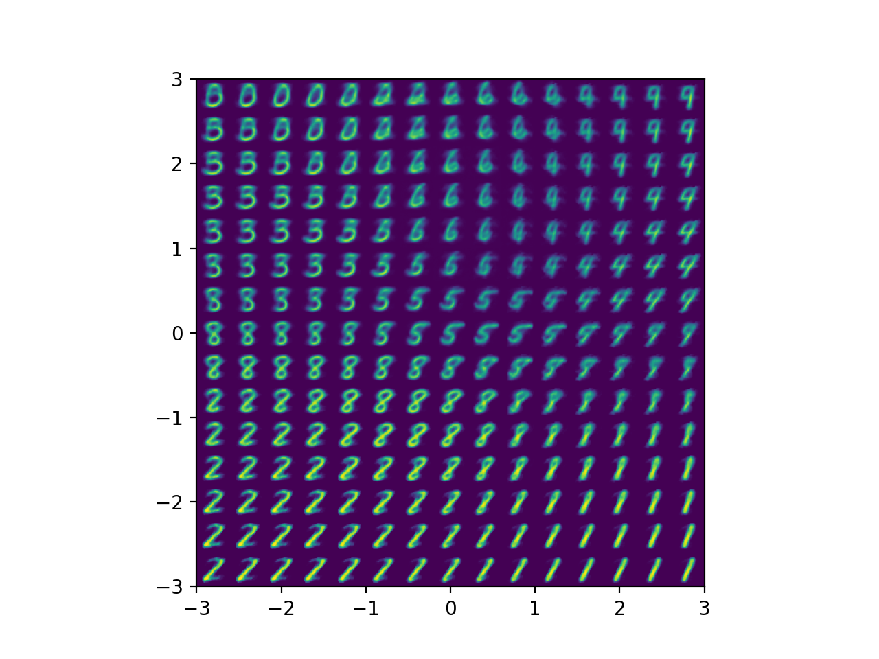 Fig. Decoded Images from 2-dim Latent Space Points (VAE)
위와 같은 사진을 얻을 수 있습니다.
(어떻게... 좀 더 잘 semantic한 걸 뽑은 것 같나요?)
사실 아직 좀 만족스럽지 않습니다.
왜냐면 저는 VAE 정도면 이정도는 해줘야 되는거 아니야? 라고 생각했기 때문인데요…
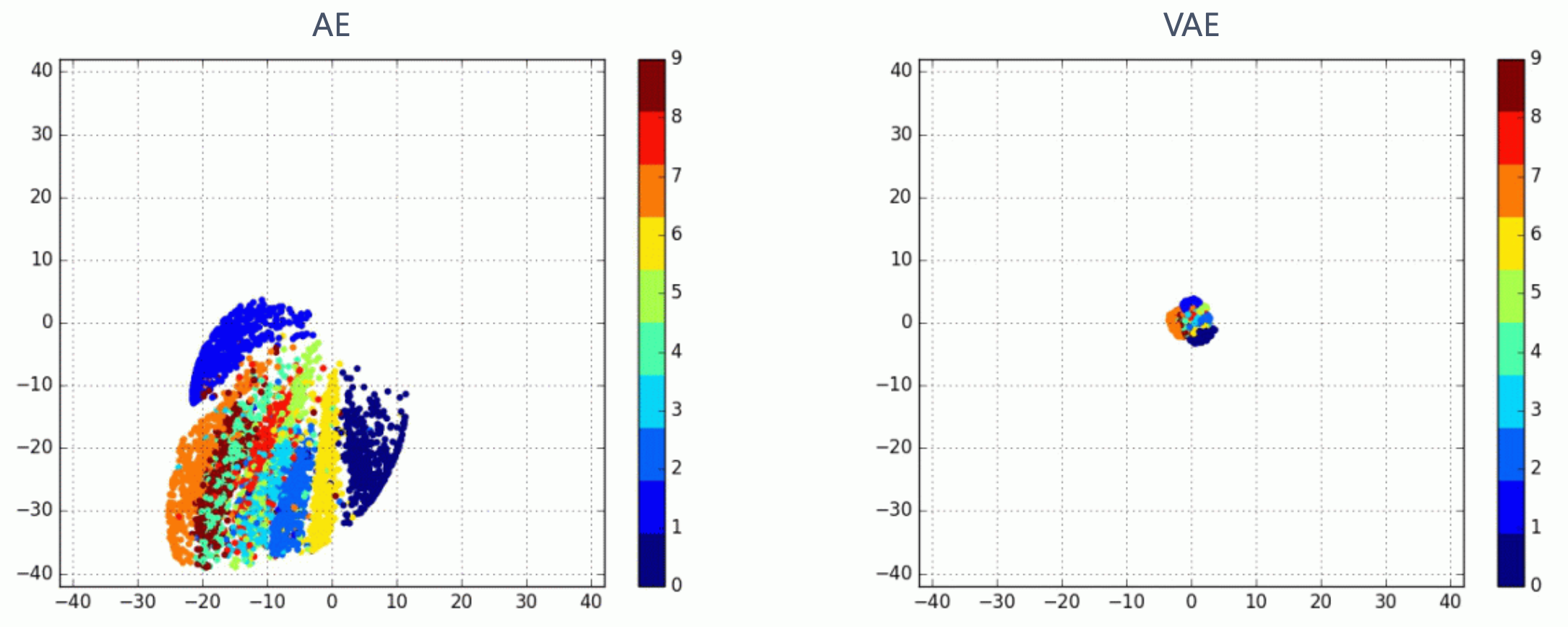 Fig. AE vs VAE Latent Space. Soruce from 오토인코더의 모든 것 (이활석님)
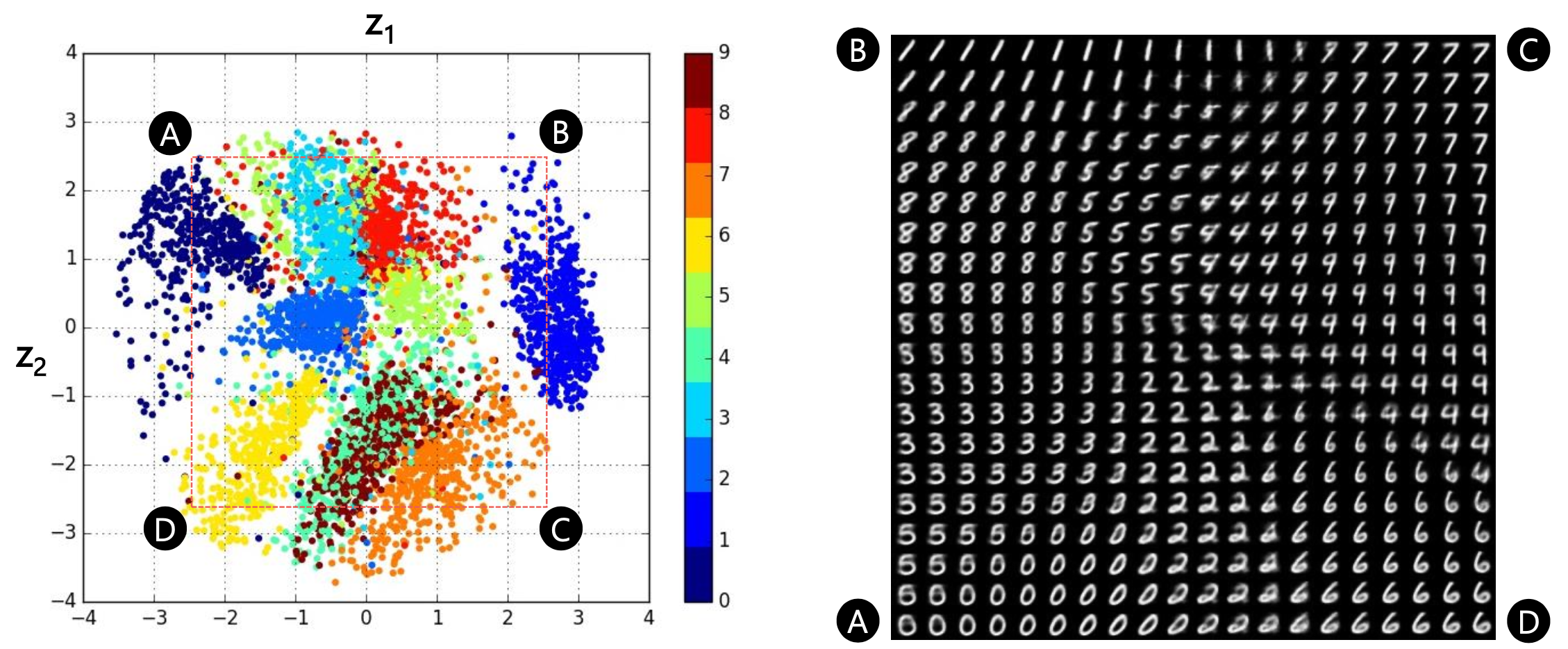 Fig. VAE Latent Space and Reconstructed Images from Latent Vectors. Soruce from 오토인코더의 모든 것 (이활석님)
그래서 모델을 CNN 섞어서 좀 깊게 만들기로 했습니다.
Encoder에 2D CNN layer를 4~5층 정도 쌓고
class DeepEncoder(nn.Module):
    def __init__(self, image_size, num_channel, latent_dims):
        super(DeepEncoder, self).__init__()

        modules = []
        hidden_dims = [32, 64, 128, 256, 512] if image_size == 64 else [64, 128, 256, 512]

        in_channel = num_channel
        for h_dim in hidden_dims:
            modules.append(
                nn.Sequential(
                    nn.Conv2d(in_channel, out_channels=h_dim,
                              kernel_size= 3, stride= 2, padding  = 1),
                    nn.BatchNorm2d(h_dim),
                    nn.LeakyReLU())
            )
            in_channel = h_dim

        self.encoder = nn.Sequential(*modules)
        self.linear_mean = nn.Linear(hidden_dims[-1]*4, latent_dims)
        self.linear_variance = nn.Linear(hidden_dims[-1]*4, latent_dims)

        self.N = torch.distributions.Normal(0, 1) # zero mean, unit variance gaussian dist

        if device == 'cuda':
            self.N.loc = self.N.loc.cuda() # hack to get sampling on the GPU
            self.N.scale = self.N.scale.cuda()

        self.kld = 0

    def forward(self, x):
        x = self.encoder(x)
        x = torch.flatten(x, start_dim=1)

        mu = self.linear_mean(x) # mean
        sigma = torch.exp(self.linear_variance(x)) # variance
        z = mu + sigma * self.N.sample(mu.shape) # sampled with reparm trick

        self.kld = (sigma**2 + mu**2 - torch.log(sigma) - 1/2).sum() # closed-form kl divergence solution

        return z
디코더도 유사하게 쌓습니다.
class DeepDecoder(nn.Module):
    def __init__(self, image_size, num_channel, latent_dims):
        super(DeepDecoder, self).__init__()

        self.image_size = image_size
        self.num_channel = num_channel

        modules = []
        hidden_dims = [512, 256, 128, 64, 32] if image_size == 64 else [512, 256, 128, 64]

        self.decoder_input = nn.Linear(latent_dims, hidden_dims[0] * 4)

        for i in range(len(hidden_dims) - 1):
            modules.append(
                nn.Sequential(
                    nn.ConvTranspose2d(hidden_dims[i],
                                       hidden_dims[i + 1],
                                       kernel_size=3,
                                       stride = 2,
                                       padding=1,
                                       output_padding=1),
                    nn.BatchNorm2d(hidden_dims[i + 1]),
                    nn.LeakyReLU())
            )
        self.decoder = nn.Sequential(*modules)

        # 28, 32 image size
        final_conv_layer =  nn.Conv2d(
            hidden_dims[-1],
            out_channels=num_channel,
            kernel_size=5 if image_size == 28 else 3 ,
            padding=0 if image_size == 28 else 1
            )
        self.final_layer = nn.Sequential(
                            nn.ConvTranspose2d(hidden_dims[-1],
                                               hidden_dims[-1],
                                               kernel_size=3,
                                               stride=2,
                                               padding=1,
                                               output_padding=1),
                            nn.BatchNorm2d(hidden_dims[-1]),
                            nn.LeakyReLU(),
                            final_conv_layer
                            )

    def forward(self, z):
        out = self.decoder_input(z)
        out = out.view(-1, 512, 2, 2)
        out = self.decoder(out)
        out = self.final_layer(out)
        out = torch.sigmoid(out)
        return out
그리고 use_deep_layers 라는 argument 로 이를 선택할 수 있게 했죠.
class VariationalAutoencoder(nn.Module):
    def __init__(self, image_size, num_channel, latent_dims, use_deep_layers):
        super(VariationalAutoencoder, self).__init__()
        if not use_deep_layers :
            self.encoder = Encoder(image_size, num_channel, latent_dims)
            self.decoder = Decoder(image_size, num_channel, latent_dims)
        else:
            self.encoder = DeepEncoder(image_size, num_channel, latent_dims)
            self.decoder = DeepDecoder(image_size, num_channel, latent_dims)

    def forward(self, x):
        z = self.encoder(x)
        return self.decoder(z)
그 결과 아래처럼 좀 더 오밀조밀한 공간, 즉 -3~3 정도로 더 좁은 공간에 embedding vector들이 매핑되는걸 볼 수 있었고,
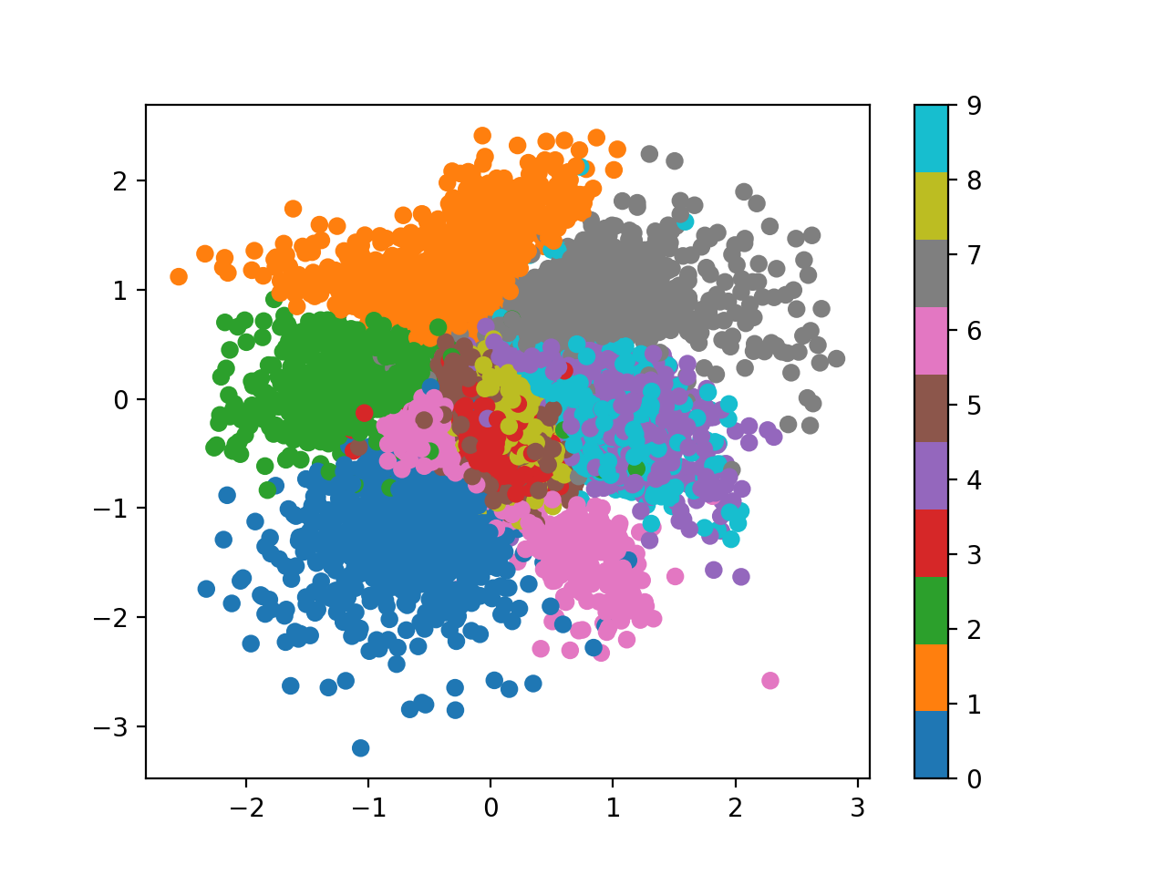 Fig.
Fig.
이 latent vector들로부터 복원한 결과도 더 깔끔한 걸 볼 수 있었습니다.
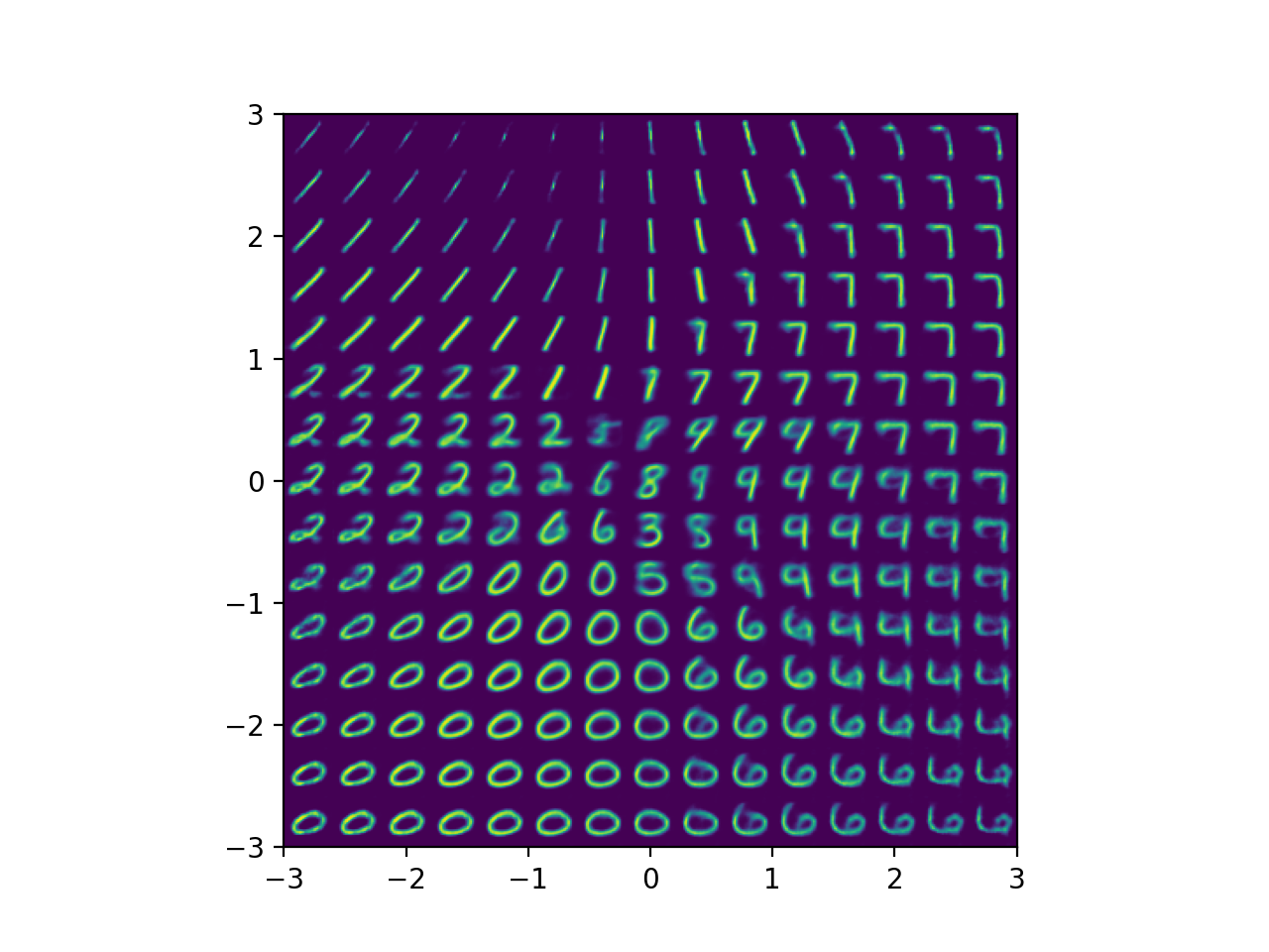 Fig.
Fig.
그리고 여기서 좀 더 나아가 원본 이미지를 Encoder -> Decoder 에 순차적으로 태워 얼마나 잘 복원하는지 확인해봤는데요,
def plot_reconstruct_from_images(model, data_loader, save_dir_path):
    og_images = None
    recon_images = None
    for i, (x,y) in enumerate(data_loader):
        og_images = x[:10]
        recon_images = model(x.to(device))[:10]
        break;

    plt.clf()
    fig, axs = plt.subplots(2, 10, figsize=(16, 6))
    for j, (og, recon) in enumerate(zip(og_images, recon_images)):
        axs[0, j].imshow(og.permute(1, 2, 0).to('cpu').detach().numpy())
        axs[1, j].imshow(recon.permute(1, 2, 0).to('cpu').detach().numpy())
        axs[0, j].axis('off')
        axs[1, j].axis('off')
    plt.tight_layout()
    plt.show()

    file_path = os.path.join(save_dir_path,'reconstruct_from_images.png')
    if os.path.exists(file_path) : os.remove(file_path)
    plt.savefig(file_path)
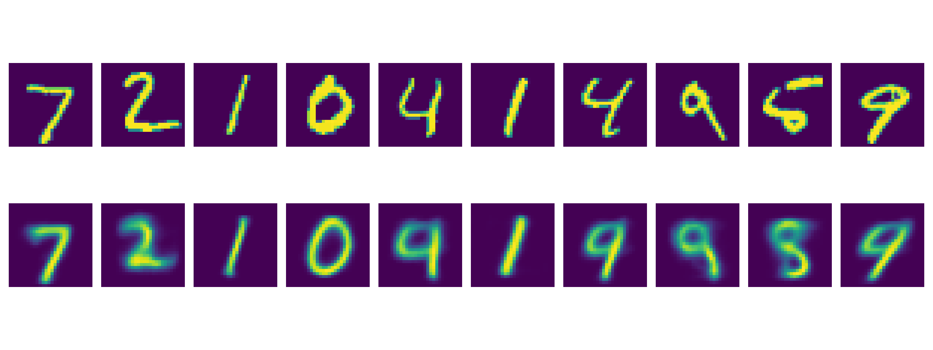 Fig.
Fig.
당연히 잘 되는걸 볼 수 있고 그 다음으로 2차원의 random vector를 생성해서 Decoder에게 이미지를 복원하라고 시켰더니
def plot_random_sample_from_prior(model, latent_dims, save_dir_path):
    z = torch.randn(10, latent_dims)
    samples = model.decoder(z.to(device))

    plt.clf()
    fig, axs = plt.subplots(1, 10, figsize=(16, 3))
    for j, sample in enumerate(samples):
        axs[j].imshow(sample.permute(1, 2, 0).to('cpu').detach().numpy())
        axs[j].axis('off')
    plt.tight_layout()
    plt.show()

    file_path = os.path.join(save_dir_path,'sample_from_prior.png')
    if os.path.exists(file_path) : os.remove(file_path)
    plt.savefig(file_path)

    return samples
이것도 잘 하는걸 볼 수 있었습니다.
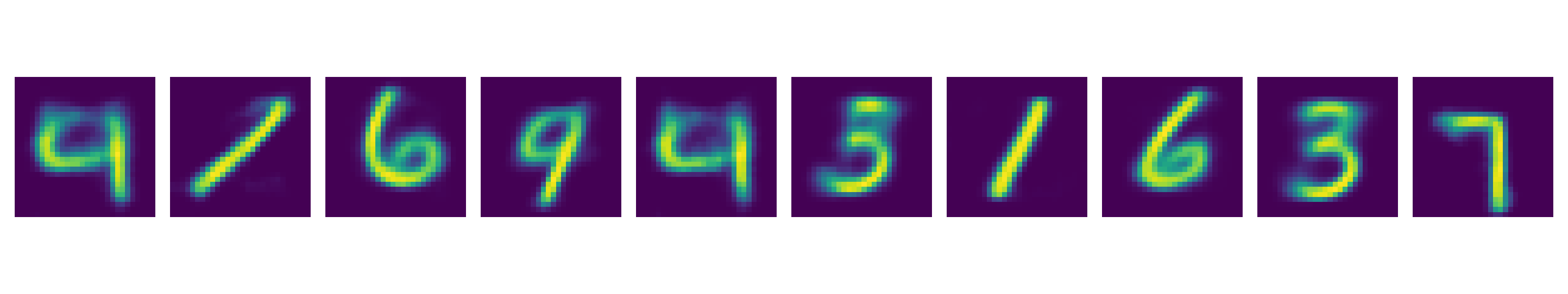 Fig.
Fig.
마지막으로 Alexander Van de Kleut가 한 것처럼 두 개의 서로다른 class로 부터 latent vector를 뽑은 뒤 이 두개의 벡터를 서로 interpolation 하는 실험을 해봤는데요,
def interpolate(model, image_size, num_channel, save_dir_path, x1, x2, n=20):
    z1 = model.encoder(x1)[0]
    z2 = model.encoder(x2)[0]

    z = torch.stack([z1 + (z2 - z1)*t for t in np.linspace(0, 1, n)])
    interpolate_list = model.decoder(z.to(device)).to('cpu').detach()

    plt.clf()
    w = image_size
    img = np.zeros((w, n*w, num_channel))
    for i, x_hat in enumerate(interpolate_list):
        x_hat = x_hat.reshape(num_channel, image_size, image_size)
        recon_img = x_hat.permute(1, 2, 0).numpy()
        img[:, i*w:(i+1)*w, :] = recon_img
    plt.imshow(img)
    plt.xticks([])
    plt.yticks([])

    file_path = os.path.join(save_dir_path,'interpolated_images.png')
    if os.path.exists(file_path) : os.remove(file_path)
    plt.savefig(file_path)
아래처럼 1과 0의 latent vector를 interpolate 하면 이상한 숫자가 decoding 되는게 아니라 embedding space상에 이 둘 사이에 매핑된 숫자들이 튀어나옵니다.
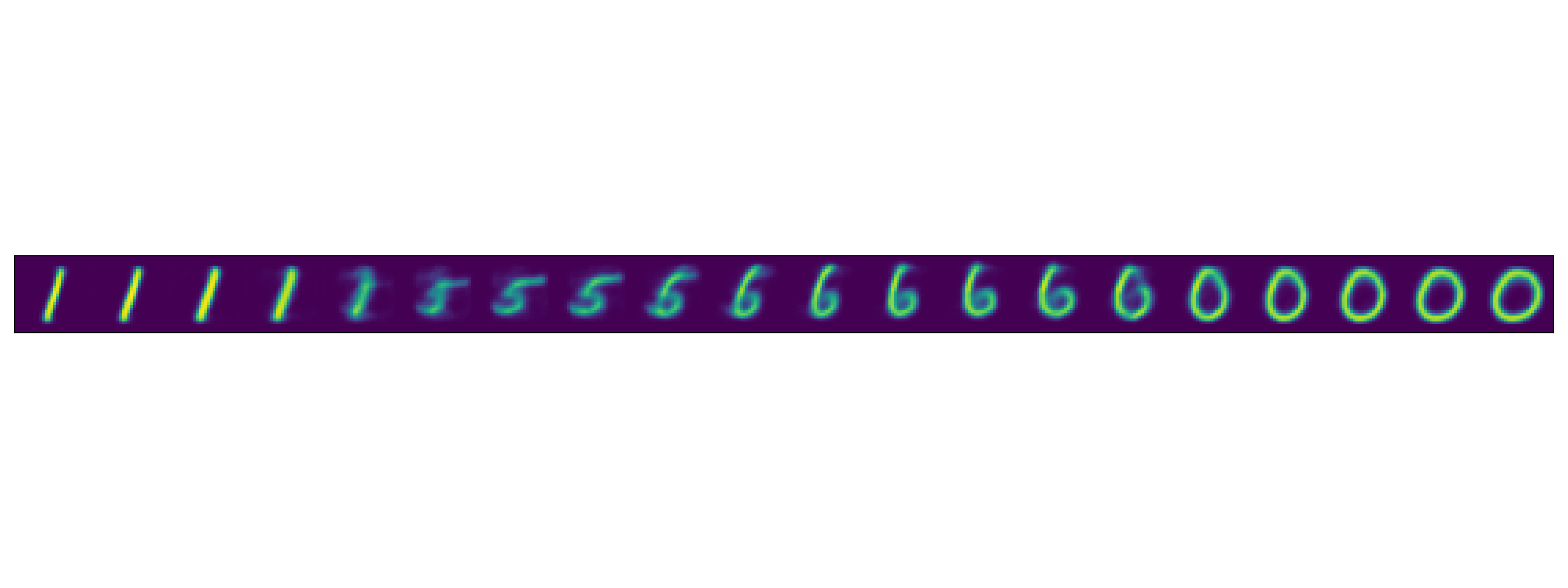 Fig.
Fig.
AE나 VAE로 학습한 인코더의 manifold가 가지는 장점은 이처럼 우리가 생각하지 못하는 데이터의 특성을 저차원에 잘 매핑시켜준다는 데 있는데요,
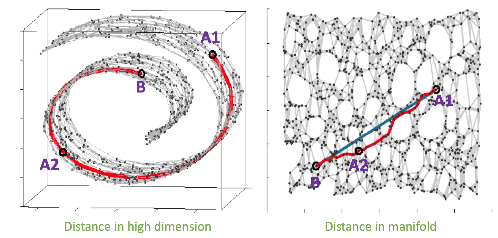 Fig.
Fig.
실제 MNIST의 원래 차원인 28*28, 즉 784차원의 고차원 공간에서는 1 과 0 (그림에서 A1과 B) 사이에 이렇다할 상관관계 등의 정보가 없었으나 (왼쪽 사진) VAE나 AE로 학습한 인코더는 이 관계를 잘 해석했기 때문에 그 사이에 A2 같은게 있다는걸 알게해준 거죠 (오른쪽 사진).
마지막으로 이 interpolation 하는 process를 애니메이션으로 표현하면
def interpolate_gif(model, image_size, num_channel, save_dir_path, x1, x2, n=100):
    z1 = model.encoder(x1)[0]
    z2 = model.encoder(x2)[0]

    z = torch.stack([z1 + (z2 - z1)*t for t in np.linspace(0, 1, n)])
    interpolate_list = model.decoder(z.to(device)).to('cpu').detach() * 255

    mode = 'F' if num_channel == 1 else 'RGB'
    trans = transforms.ToPILImage(mode)
    images_list = []
    for x_hat in interpolate_list:
        recon_img = x_hat.reshape(num_channel, image_size, image_size)
        img = (trans(recon_img)).resize((256, 256))
        # recon_img = x_hat.reshape(num_channel, image_size, image_size)[0]
        # img2 = Image.fromarray(recon_img.numpy()).resize((256, 256))
        images_list.append(img)
    images_list = images_list + images_list[::-1] # loop back beginning

    plt.clf()
    file_path = os.path.join(save_dir_path,'interpolated_images.gif')
    if os.path.exists(file_path) : os.remove(file_path)

    images_list[0].save(
        file_path,
        save_all=True,
        append_images=images_list[1:],
        loop=1)
아래처럼 좀 있어보이는 gif 파일을 얻을 수 있습니다.
 Fig.
Fig.
추가적으로 Deep CNN VAE 에 latent dimension을 128로도 키워봤는데요, 이 때는 2차원일때와 다르게 시각화 하기 힘들기 때문에 t-SNE 를 사용해서 시각화를 했습니다.
def plot_latent_with_tsne(model, data_loader, save_dir_path, dim=2):
    plt.clf()

    latents = torch.Tensor()
    labels = torch.Tensor()
    for i, (x, y) in enumerate(data_loader):
        # z = model.encoder(x.to(device)).to('cpu').detach().numpy()
        z = model.encoder(x.to(device))
        latents = torch.cat((latents,z.to('cpu')),0)
        labels = torch.cat((labels,y),0)

    z = latents.to('cpu').detach().numpy()
    y = labels.to('cpu').detach().numpy()

    tsne_vector = manifold.TSNE(
        n_components=dim, learning_rate="auto", perplexity=40, init="pca", random_state=0
    ).fit_transform(z)

    if dim == 2:
        plt.scatter(tsne_vector[:, 0], tsne_vector[:, 1], c=y, cmap='tab10')
    elif dim == 3:
        fig = plt.figure()
        ax = fig.add_subplot(projection='3d')
        ax.scatter(tsne_vector[:, 0], tsne_vector[:, 1], tsne_vector[:, 2], c=y, cmap='tab10')

    file_path = os.path.join(save_dir_path,'latent_space_with_tsne_{}d.png'.format(dim))
    if os.path.exists(file_path) : os.remove(file_path)
    plt.savefig(file_path)
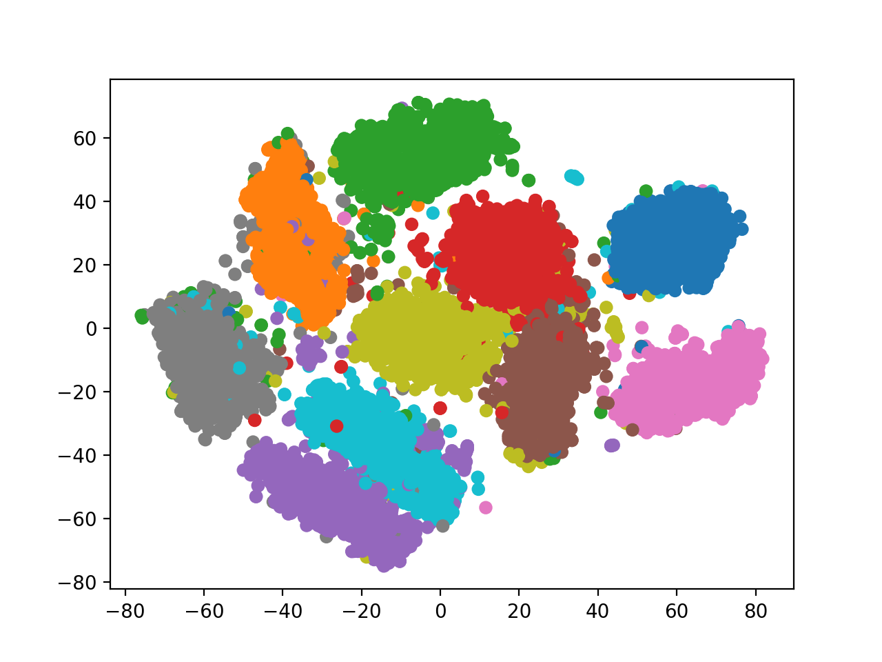 Fig. 128차원 -> 2차원 latent space 시각화
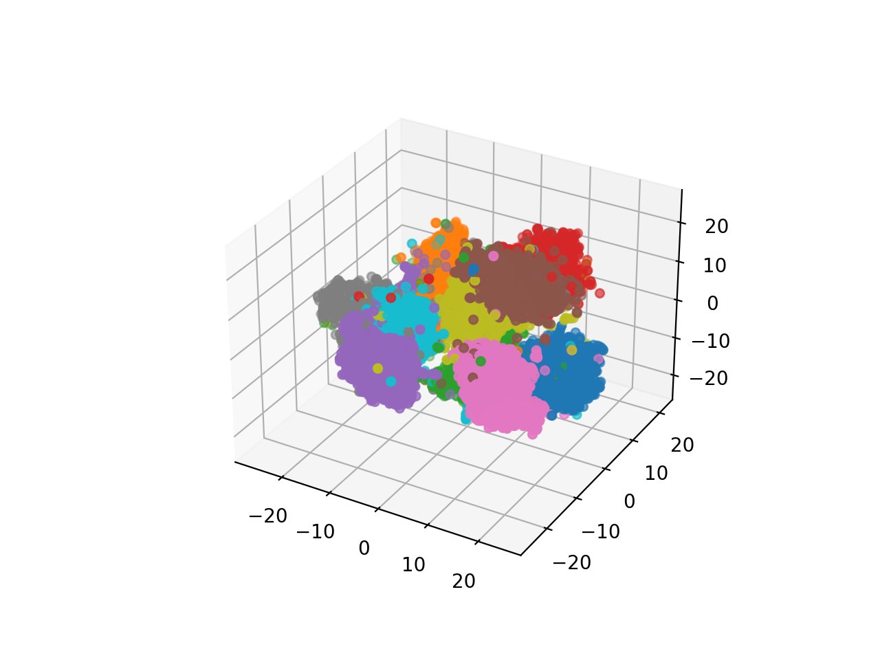 Fig. 128차원 -> 3차원 latent space 시각화
2차원일때보다 더 잘 클러스터링 된 걸 알 수 있었으나 랜덤으로 샘플링한 128차원 벡터를 디코딩 했을 때는 너무 고차원 상에 sparse하게 데이터가 매핑돼서 그런지 썩 좋지 못한 모습을 보였습니다.
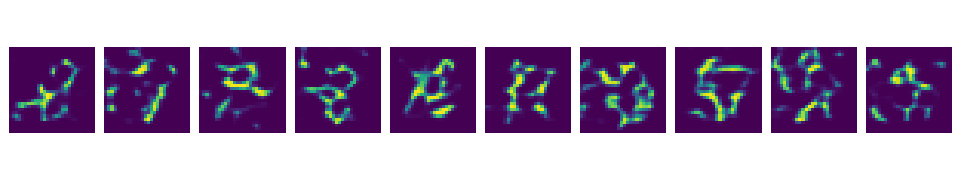 Fig. decoding random sampled 128 dim latent vector
Vector Quantized Variational AutoEncoder (VQ-VAE)
- TBC (let’s check this)