(WIP) (Preliminaries for ML) Linear Algebra
29 Mar 2023< 목차 >
- Why LinAlg ?
- Linear Combinations
- Linear Transformations
- Matrix Multiplication
- Three-dimensional Linear Transformations
- The Determinant
- Inverse matrices, column space and null space
- Nonsquare matrices as transformations between dimensions
- Dot products and duality
- Cross products
- Cross products in the light of linear transformations
- Cramer's rule, explained geometrically
- Change of basis
- Eigenvectors and eigenvalues
- A quick trick for computing eigenvalues
- Singular Value Decomposition (SVD)
- Abstract vector spaces
- References
본 Post 는 3Blue1Brown (3B1B) 의 Video 들을 기반으로 만들어졌습니다.
Why LinAlg ?
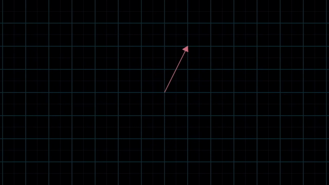
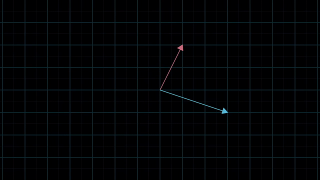
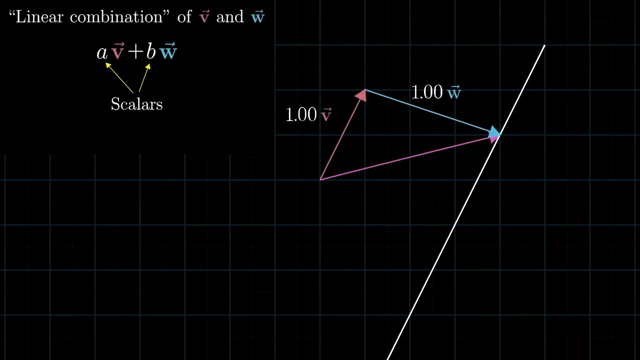
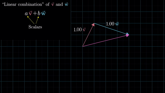
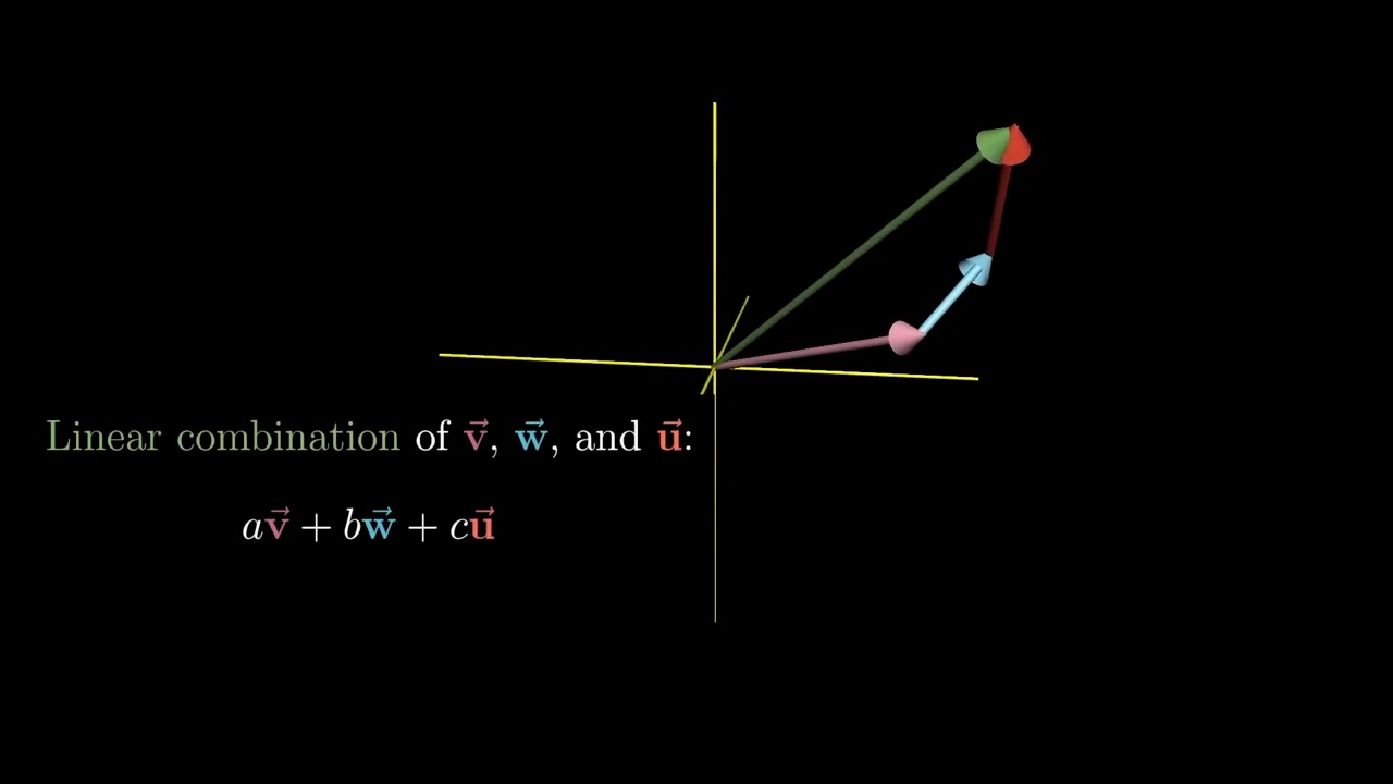
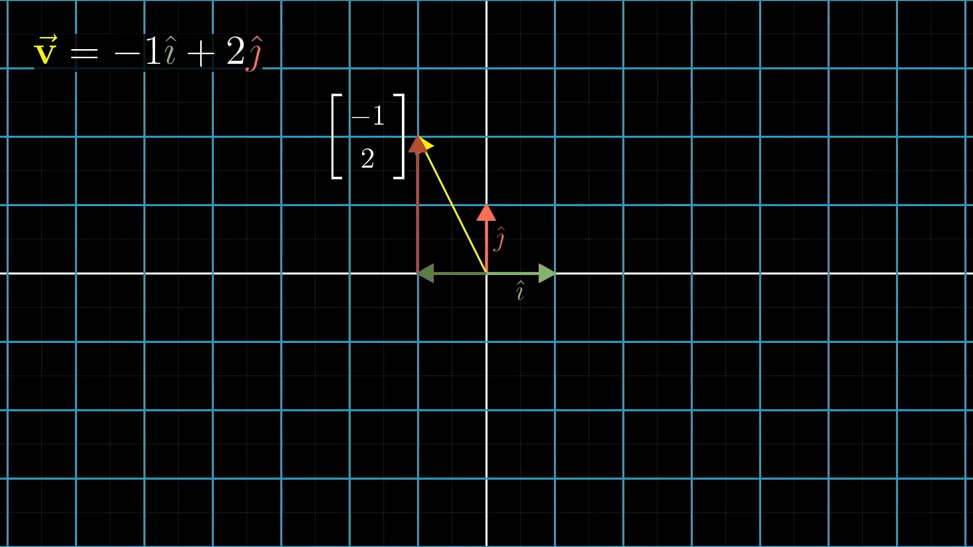
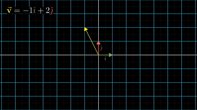
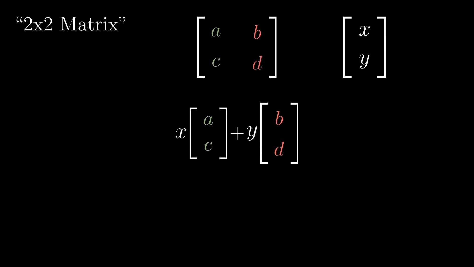
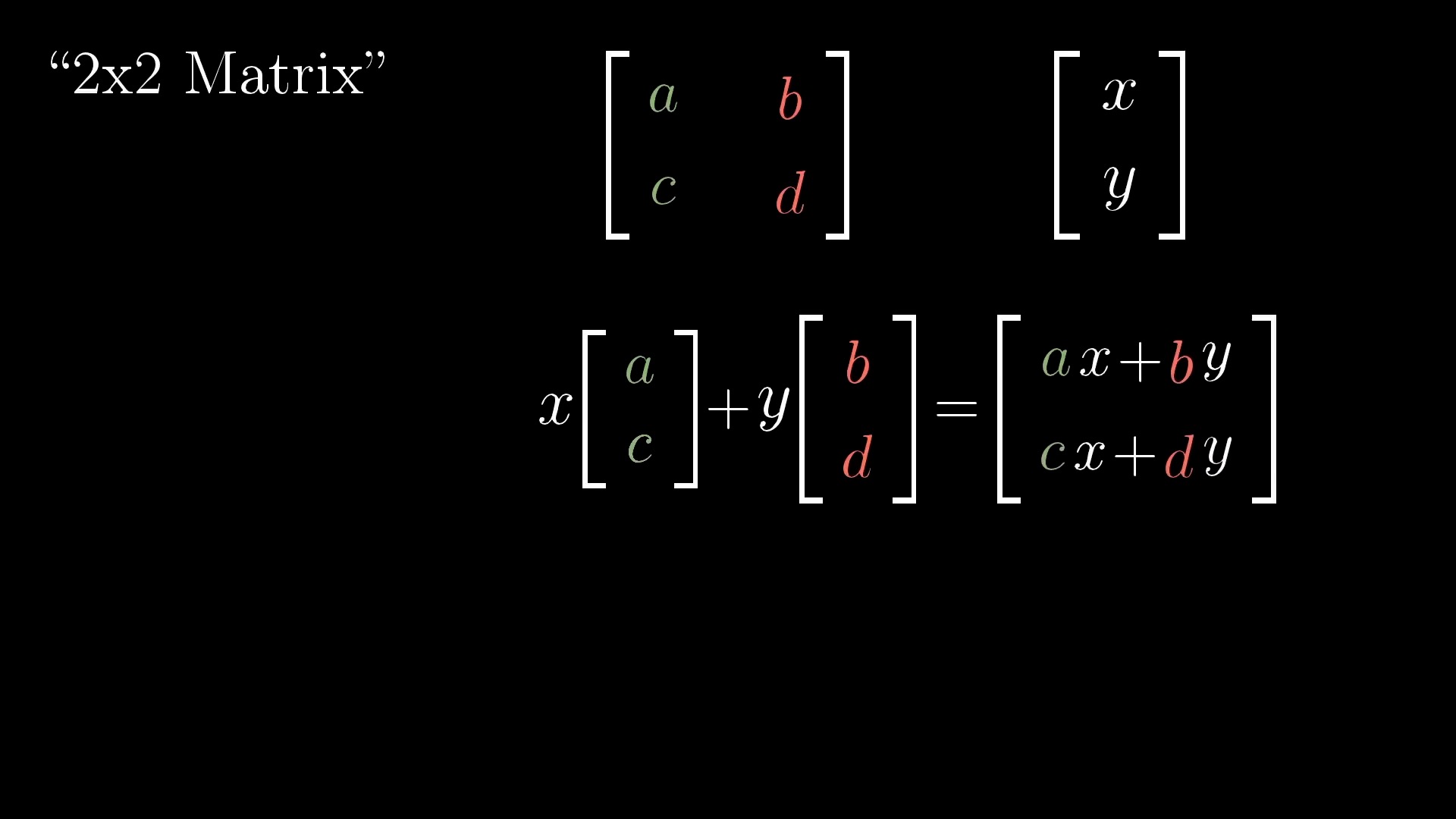
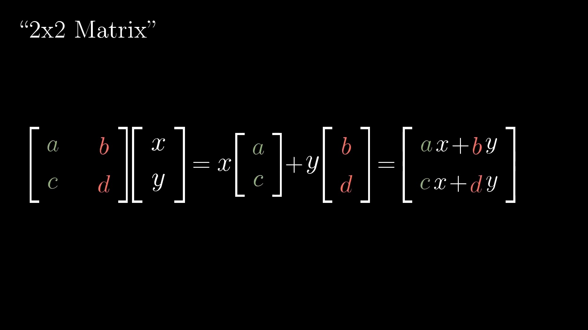
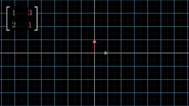
Linear Combinations
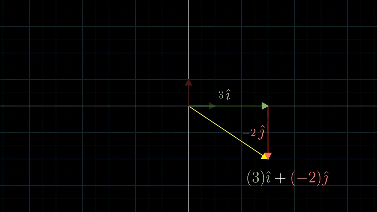
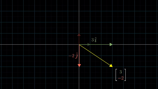
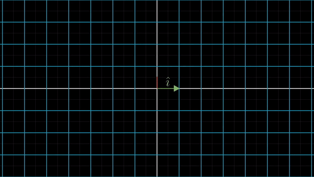
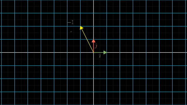
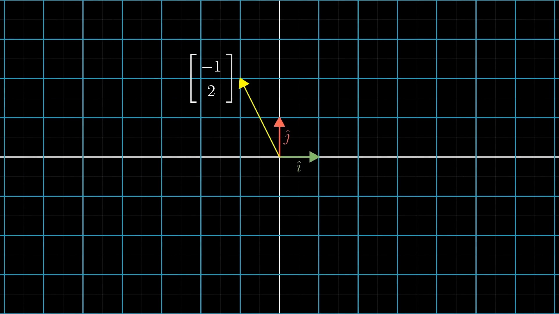
Basis Vector
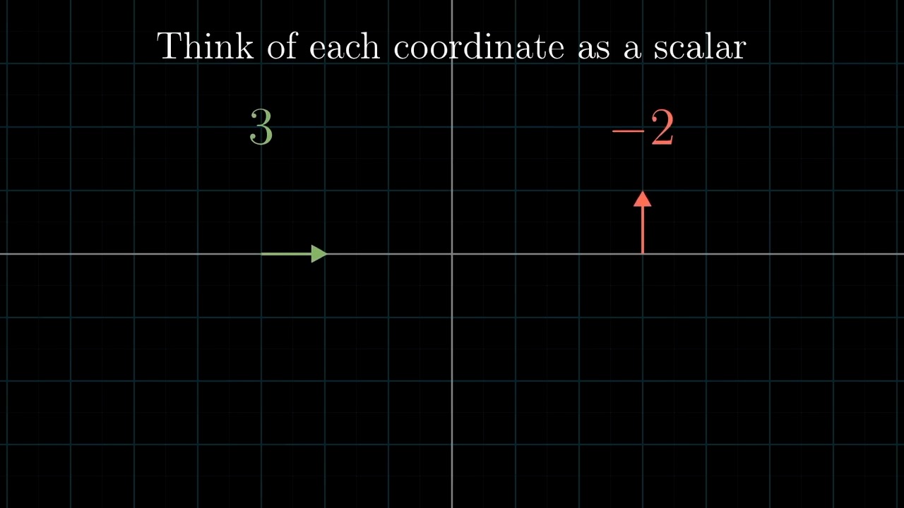
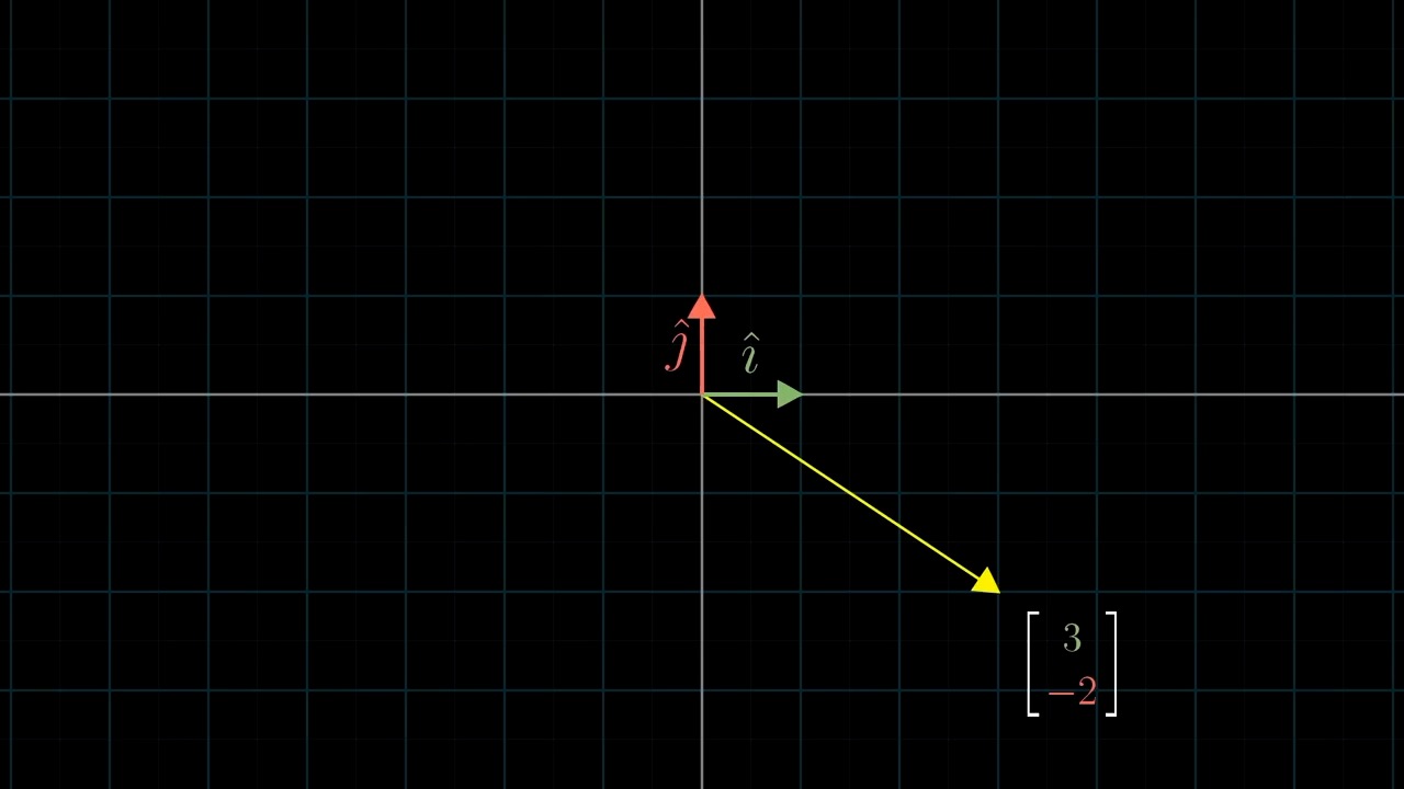
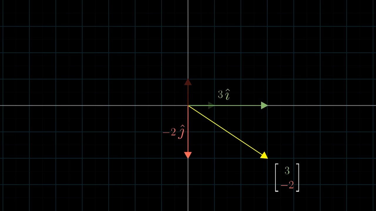
먼저 Linear Algebra 를 잘 이해하기 위해서는 어떤 특정 Vector 를 대할때 이를 어떤 기저 벡터 (Basis Vector) 의 결합으로 생각하는 것이 중요합니다.
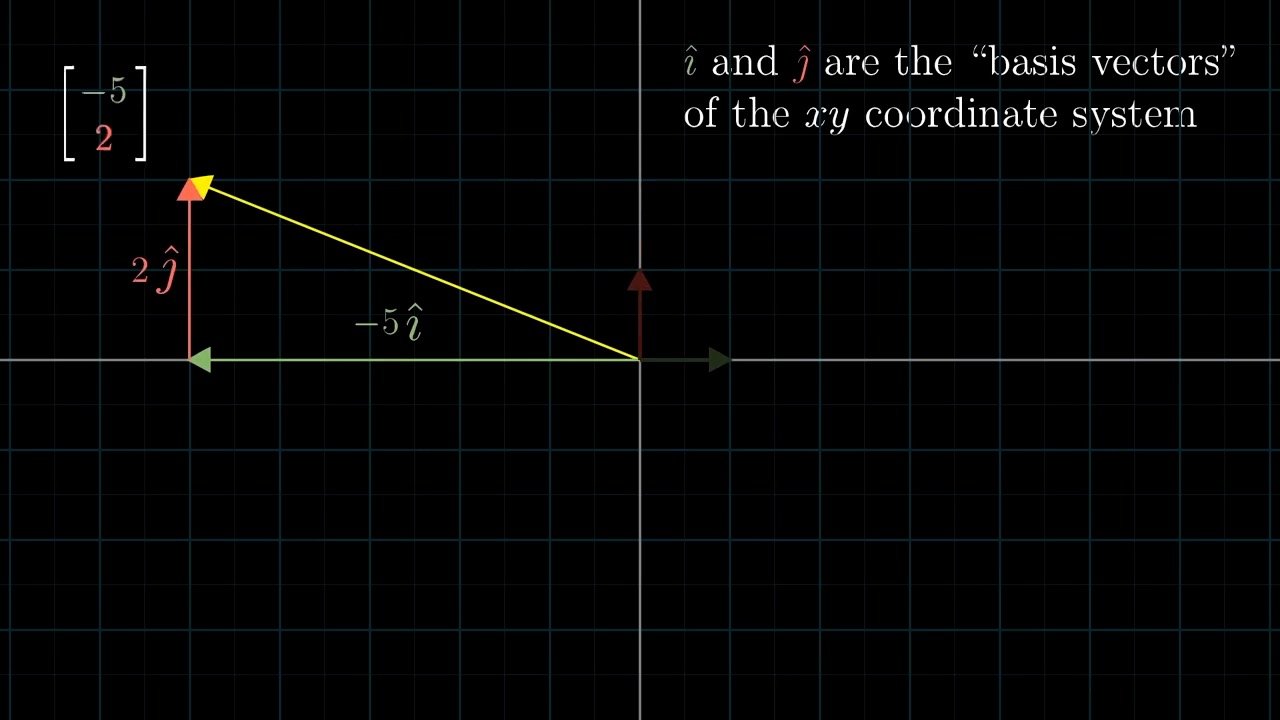
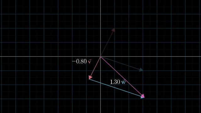
Different Basis Vector
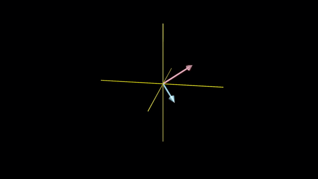
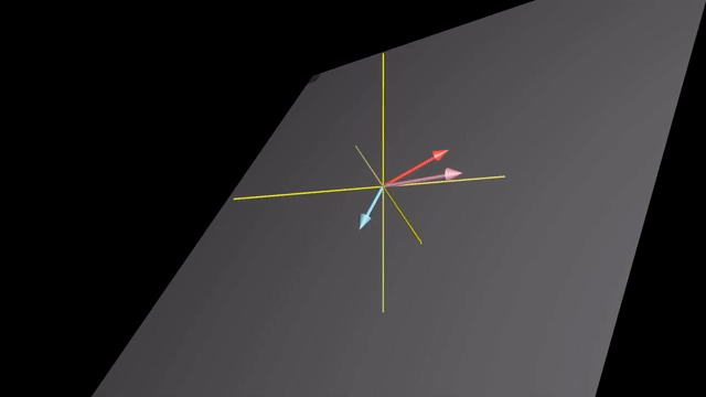
Span
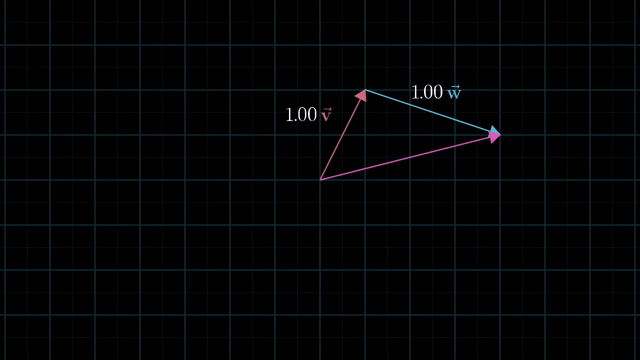
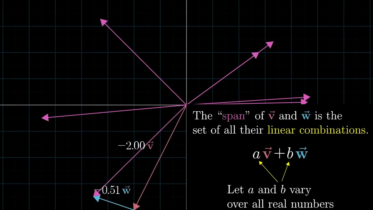
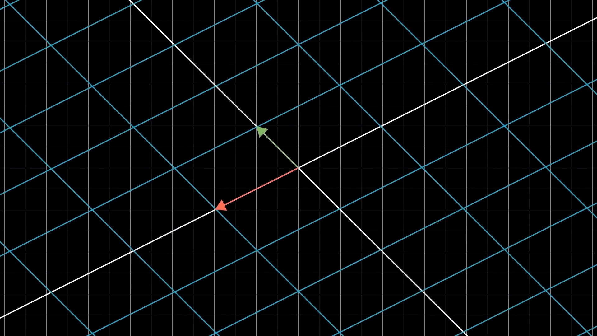
Meaning of Linear Combination
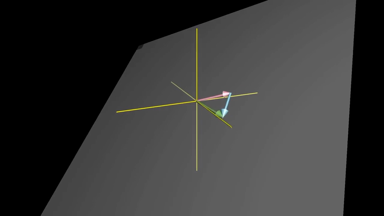
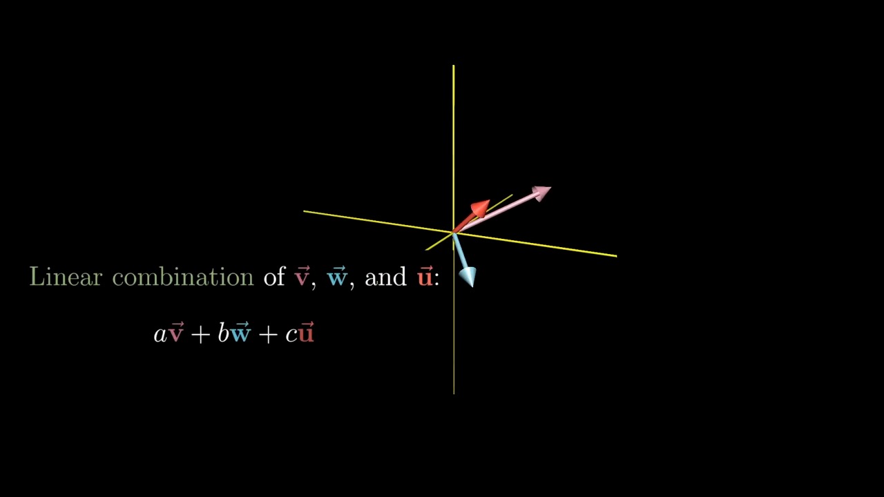
Span in 3D
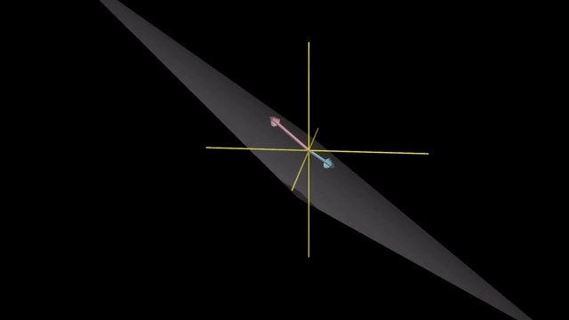
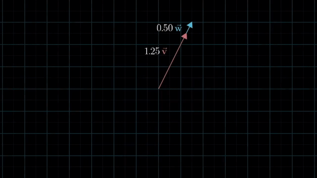
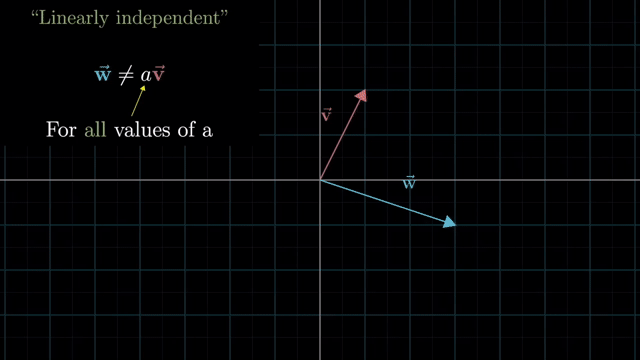
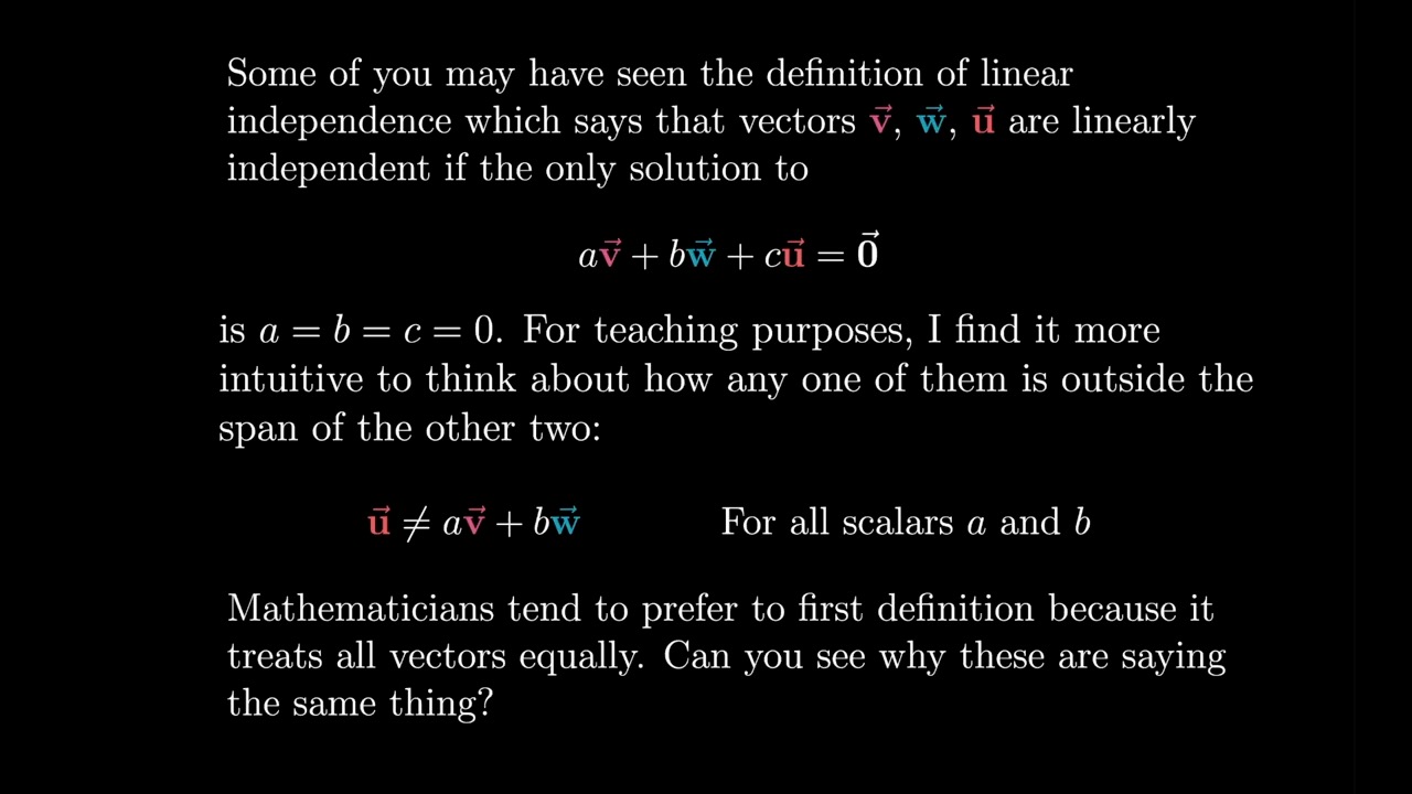
Linearly Dependent and Independent
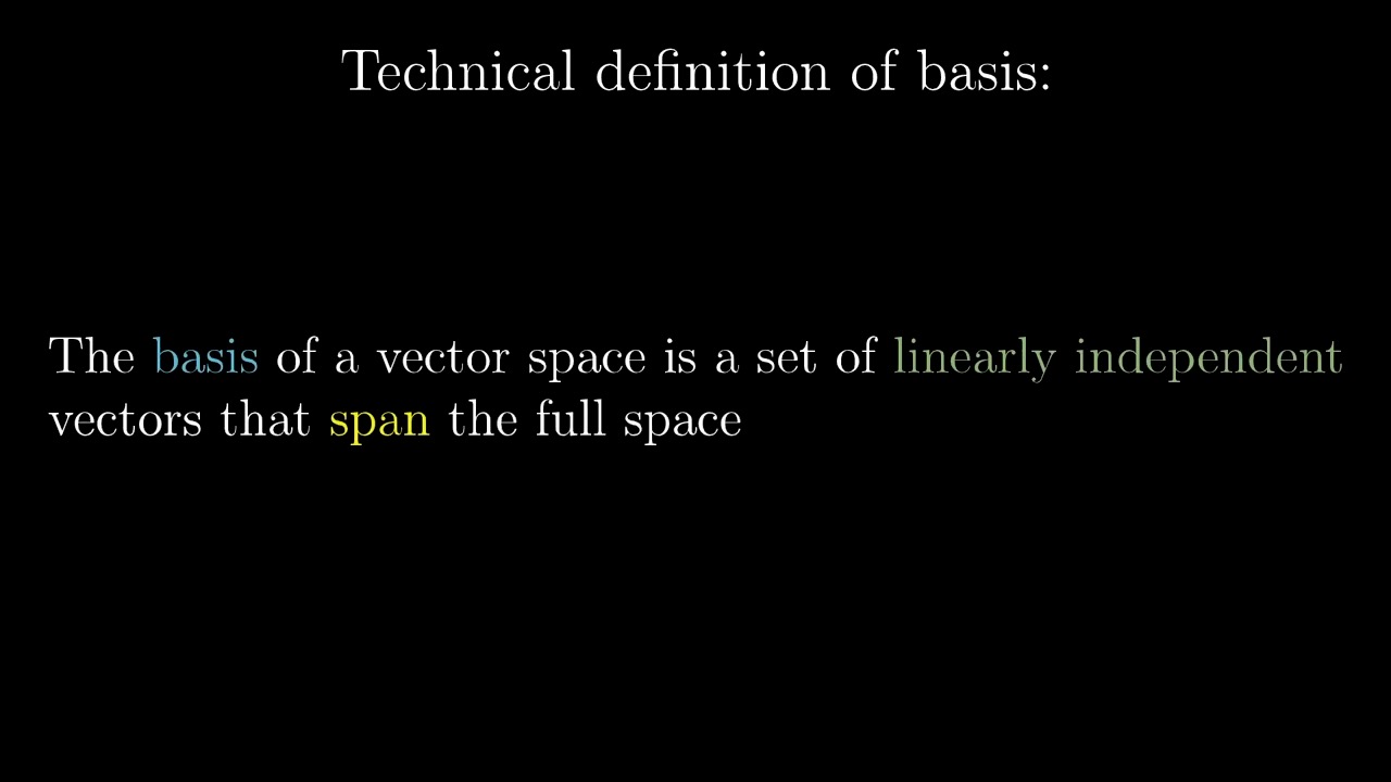
Basis Vector (Definition)
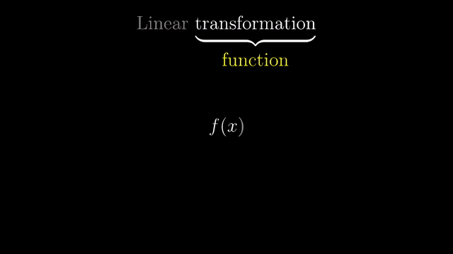
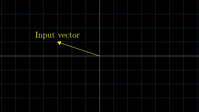
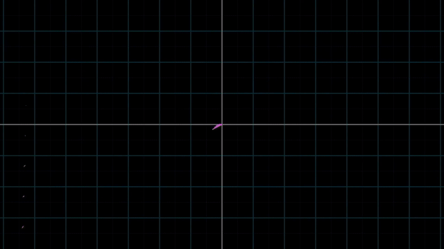
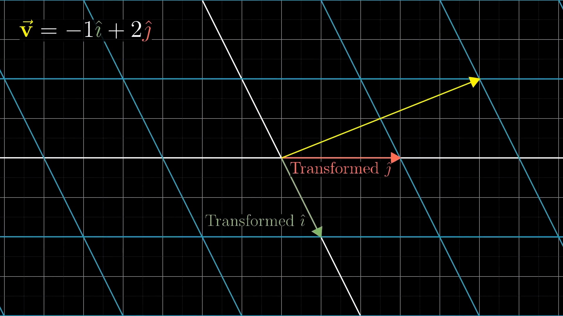
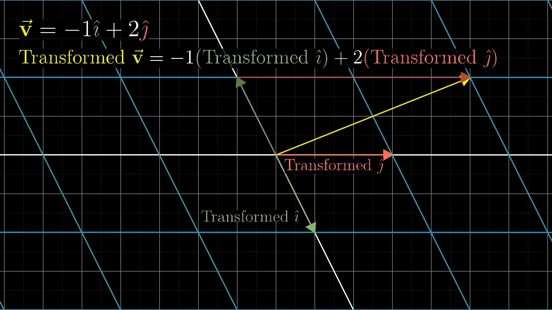
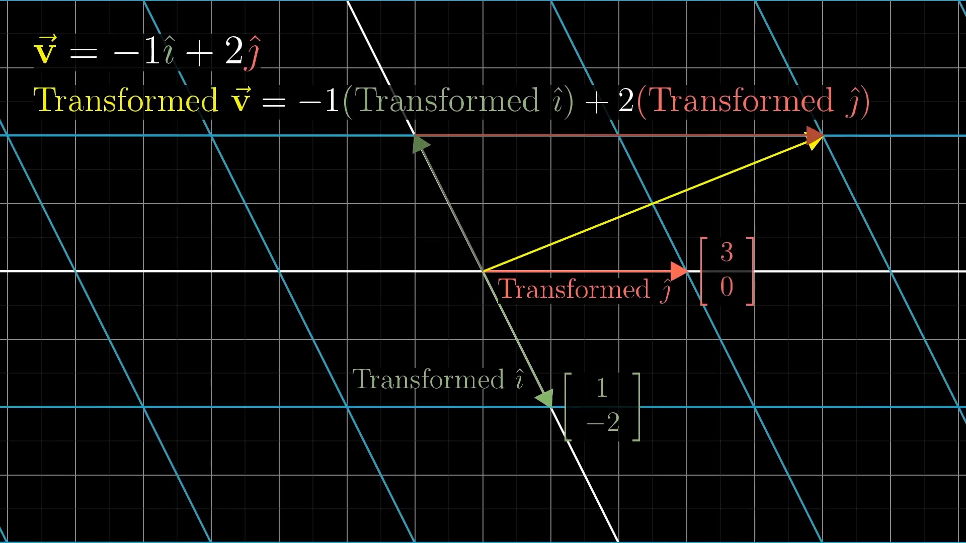
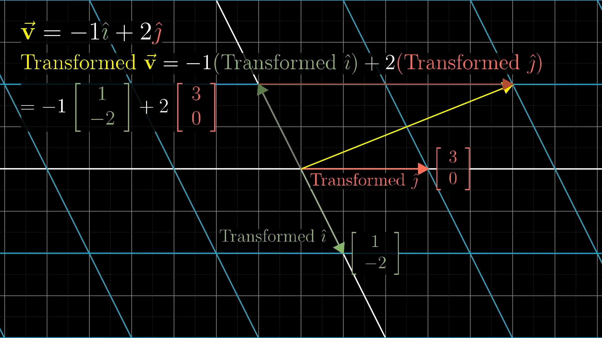
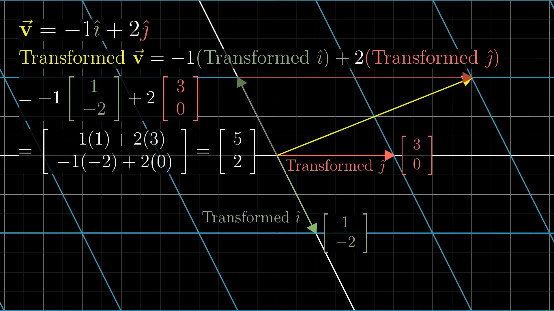
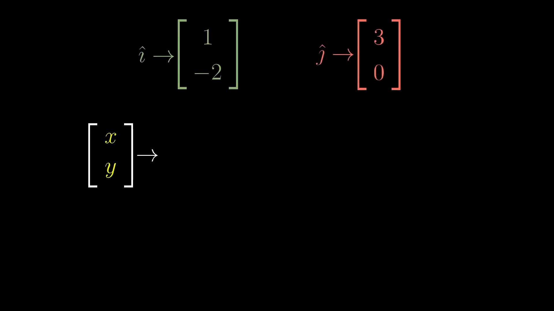
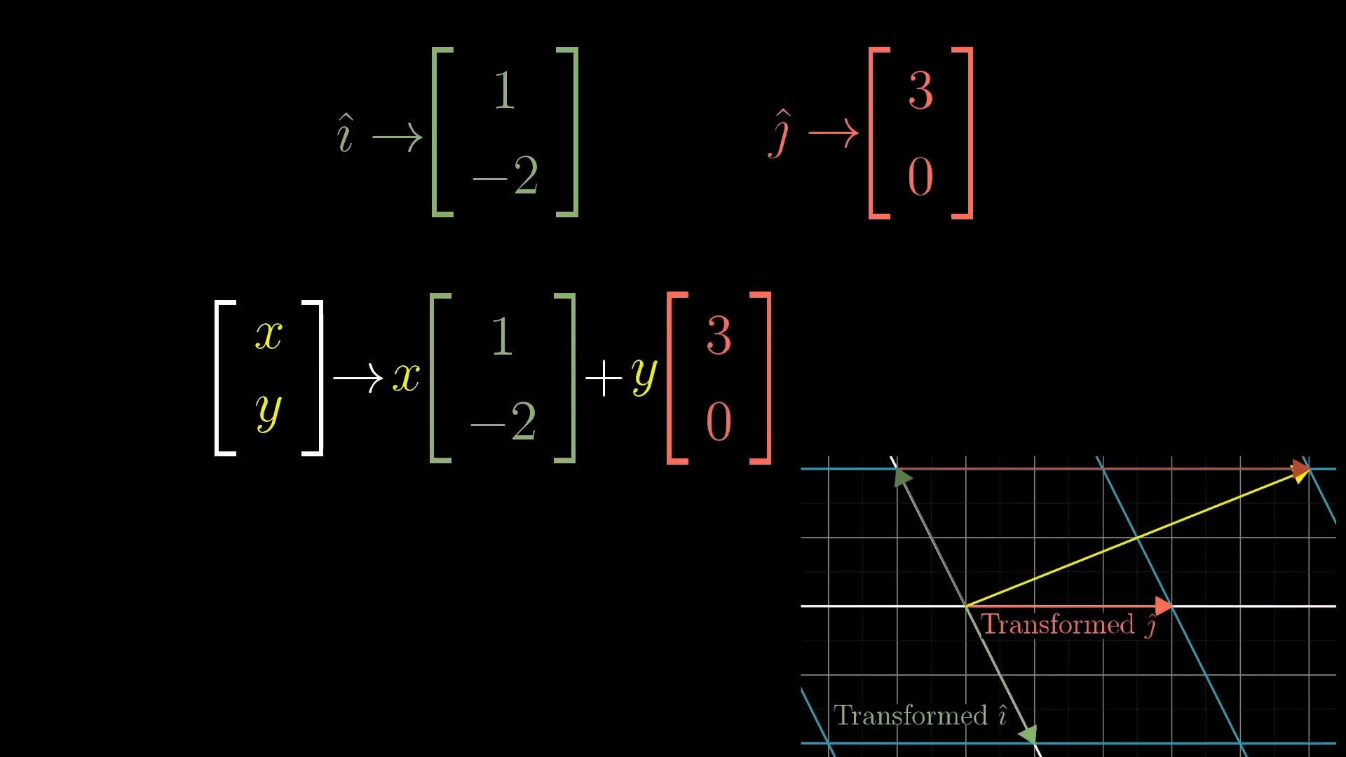
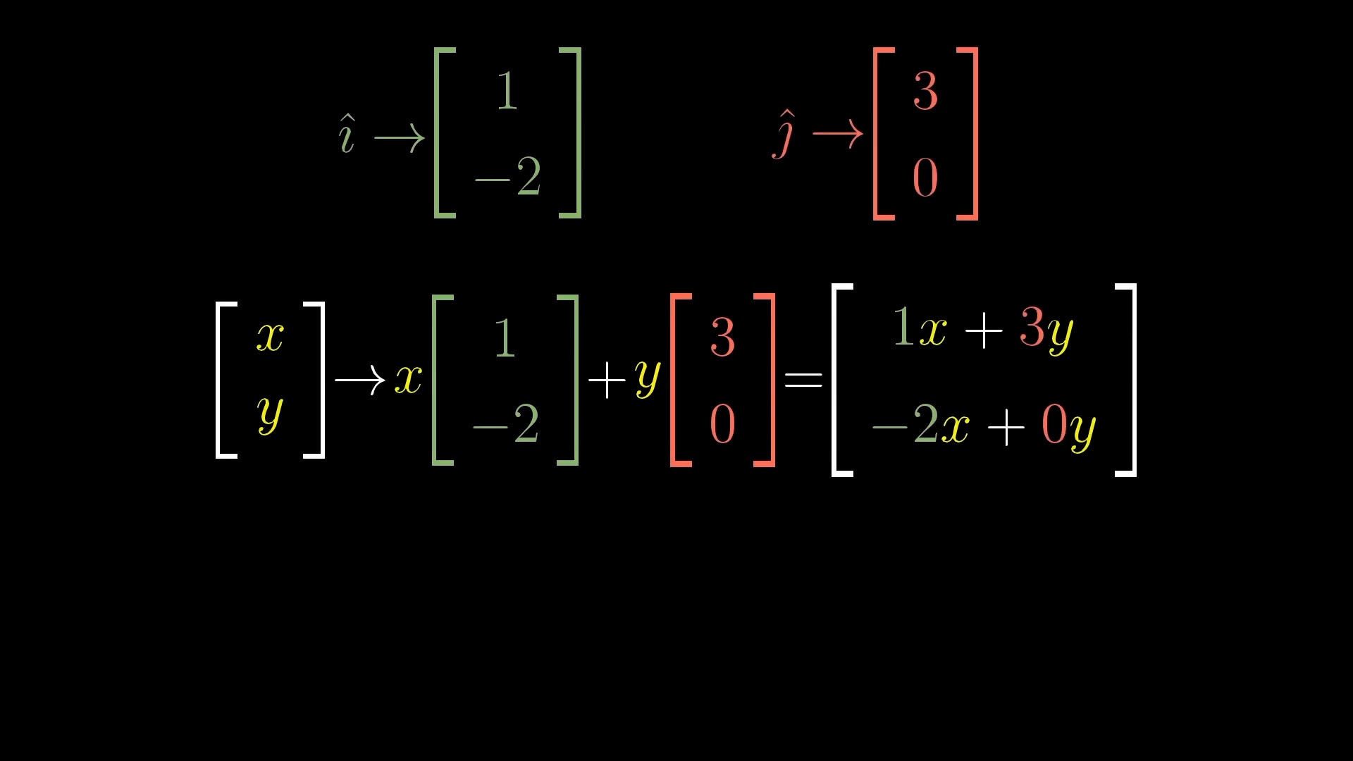
Linear Transformations
Linear Transformation is Function
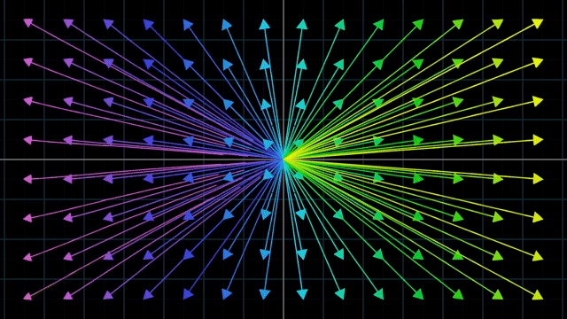
Linear vs Nonlinear Transformation Examples
반면 아래의 그림처럼 변환을 시키는 것은 선형 변환에 해당되지 않습니다. 이들은 각각의 이유로 선형 변환이라고 할 수 없는데요,
첫 번째 예시는 변형된 선들이 구부러져서 이며,
두 번째 예시는 원점이 움직여서 그렇습니다.
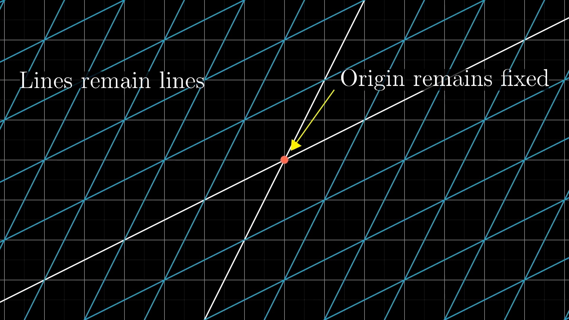
아래의 예시는 원점도 움직이지 않았고 변형된 선 또한 구부러지지 않았으나
어떤 원점을 가로지르는 직선이 있다고 칠 때 이를 선형으로 보존할 수 없게 되므로 선형 변환이 아닌것이 됩니다.
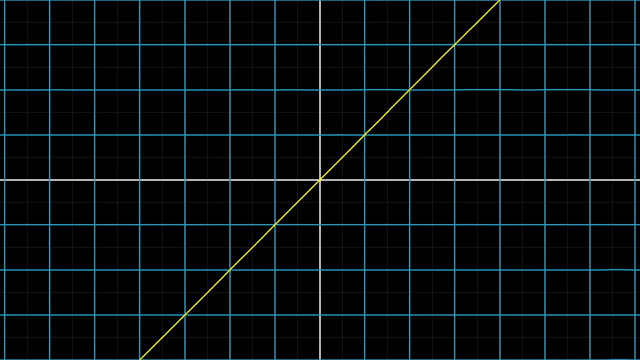
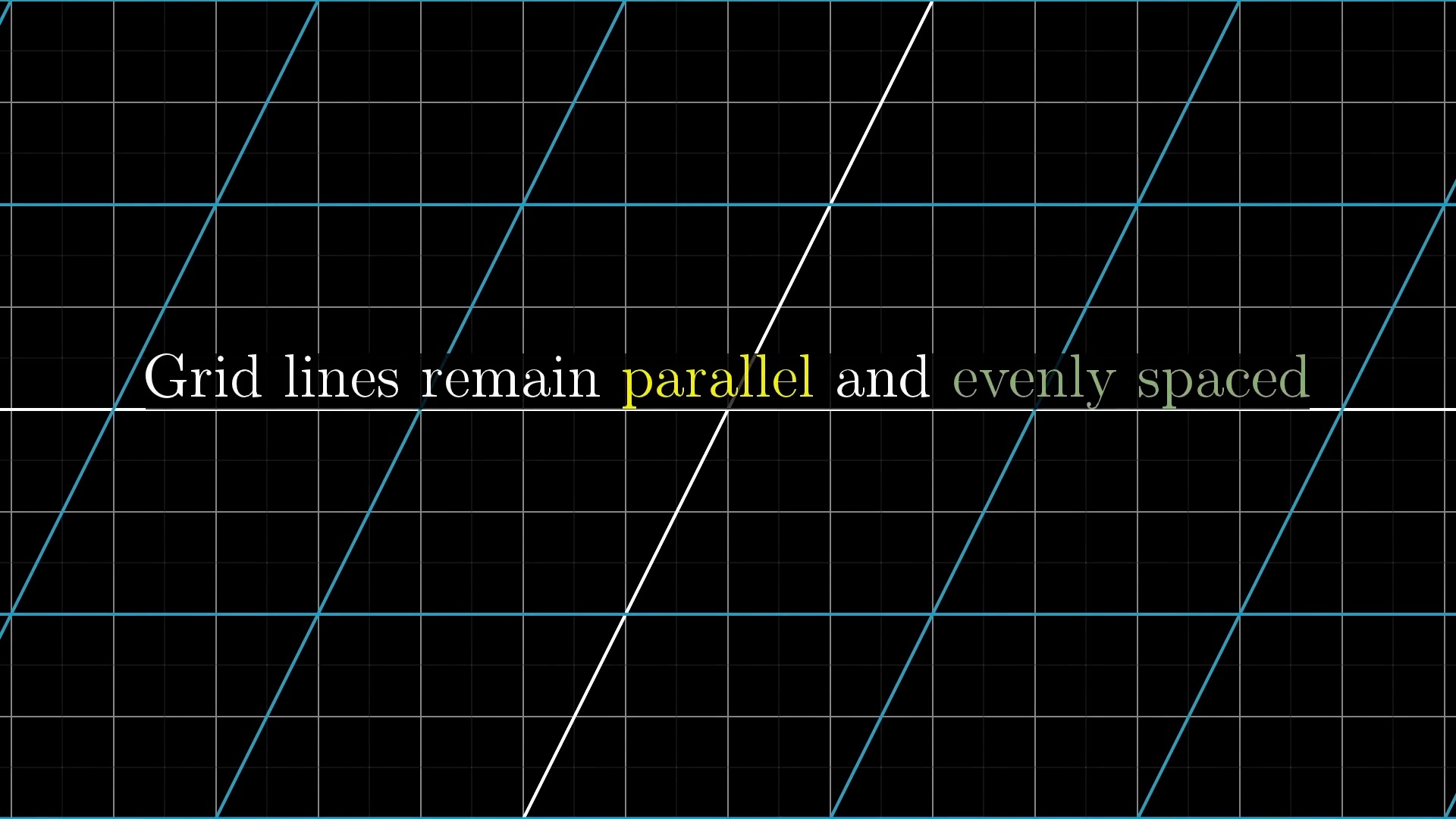
이처럼 격자 선 (Grid line) 들이 변환 후에도 여전히 평행해야 하고 (not curved) 그 격자간의 간격이 균일해야만 (evenly spaced) 선형 변환이라고 할 수 있겠습니다.
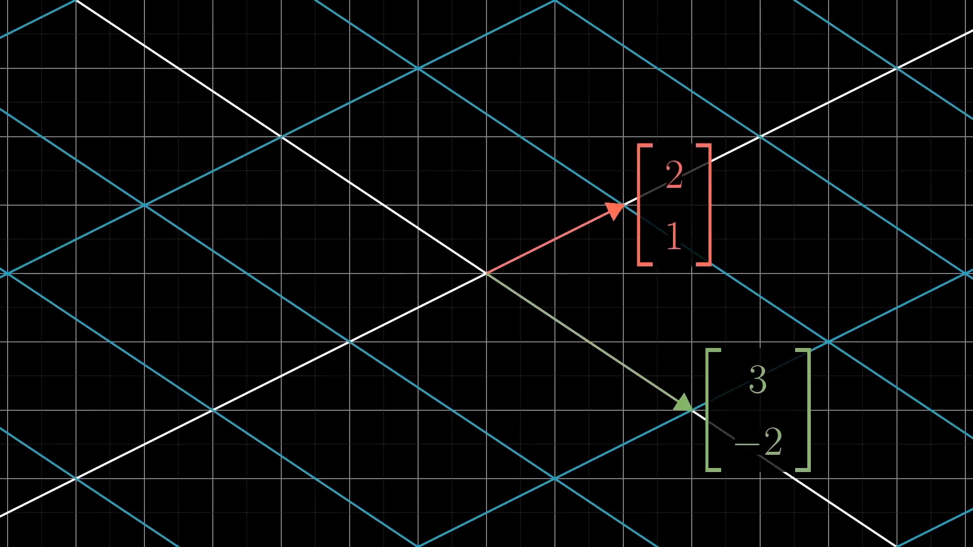
Intuitive Perspective of Linear Transformation (Change of Basis Vectors)
asd
asd
asd
asd
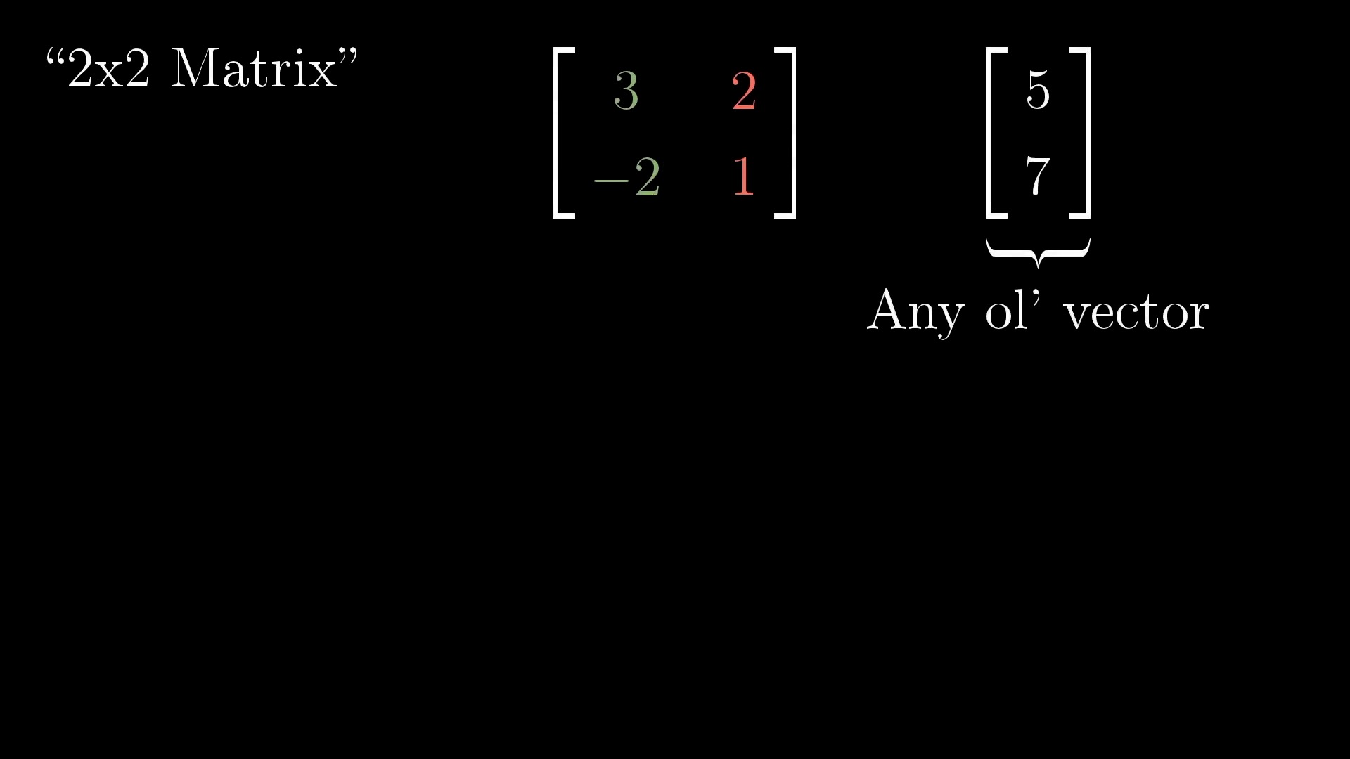
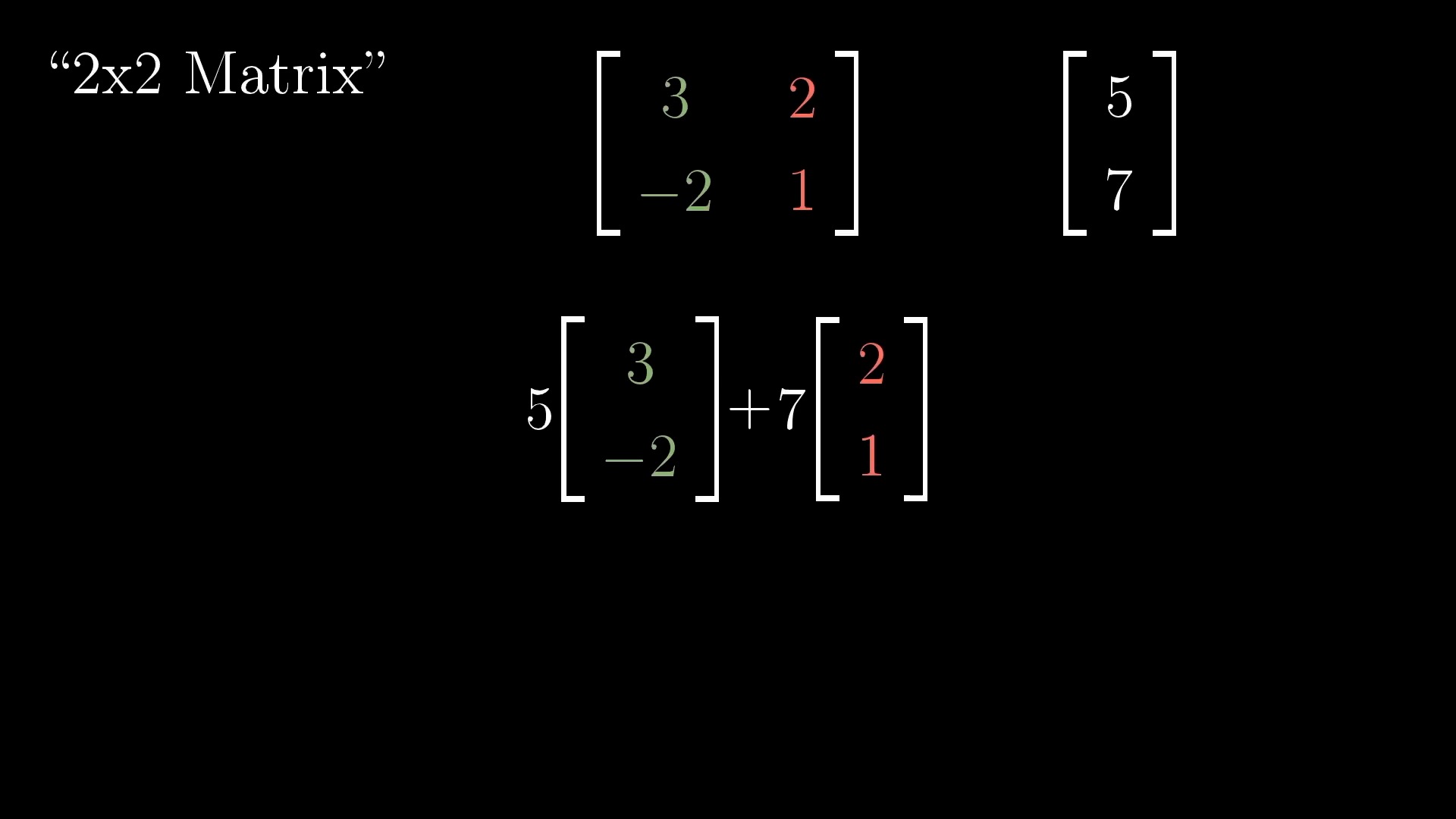
Linear Transformation (Matrix Form)
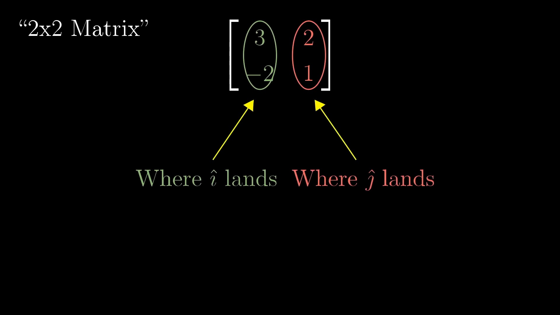
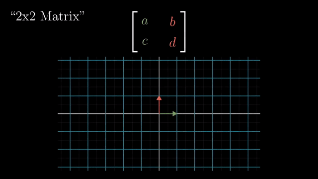
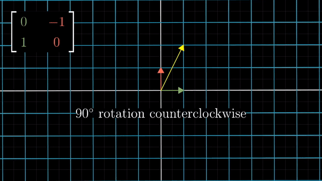
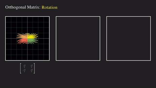
Rotation
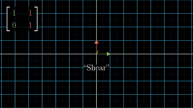
Shear
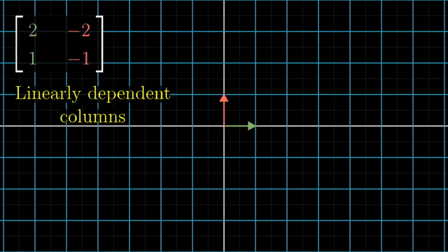
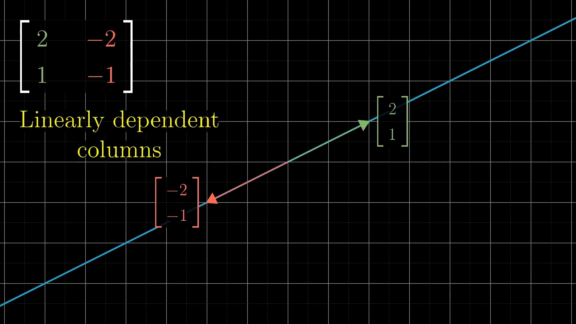
What if Rank of Transformation Matrix is Low? (Linearly Dependent)
Matrix Multiplication
Three-dimensional Linear Transformations
The Determinant
Inverse matrices, column space and null space
Nonsquare matrices as transformations between dimensions
Dot products and duality
Cross products
Cross products in the light of linear transformations
Cramer's rule, explained geometrically
Change of basis
Eigenvectors and eigenvalues
Eigen Valude Decomposition`
A quick trick for computing eigenvalues
Singular Value Decomposition (SVD)
- SVD Visualized, Singular Value Decomposition explained, SEE Matrix , Chapter 3
- What is the Singular Value Decomposition?
특이값 분해 (Singular Value Decomposition; SVD) 는 Linear Algebra 에서 굉장히 중요하며 대부분의 연산이 행렬 곱으로 이루어진 Machine Learning 알고리즘들에서 굉장히 중요한 역할을 합니다.
SVD는 어떤 행렬 \(A\)가 어떻게 생겼든지 (정사각 행렬이 아닌 경우에도) 그 행렬을 아주 생각하기 쉬운 세 가지 행렬로 분해할 수 있게 해줍니다.
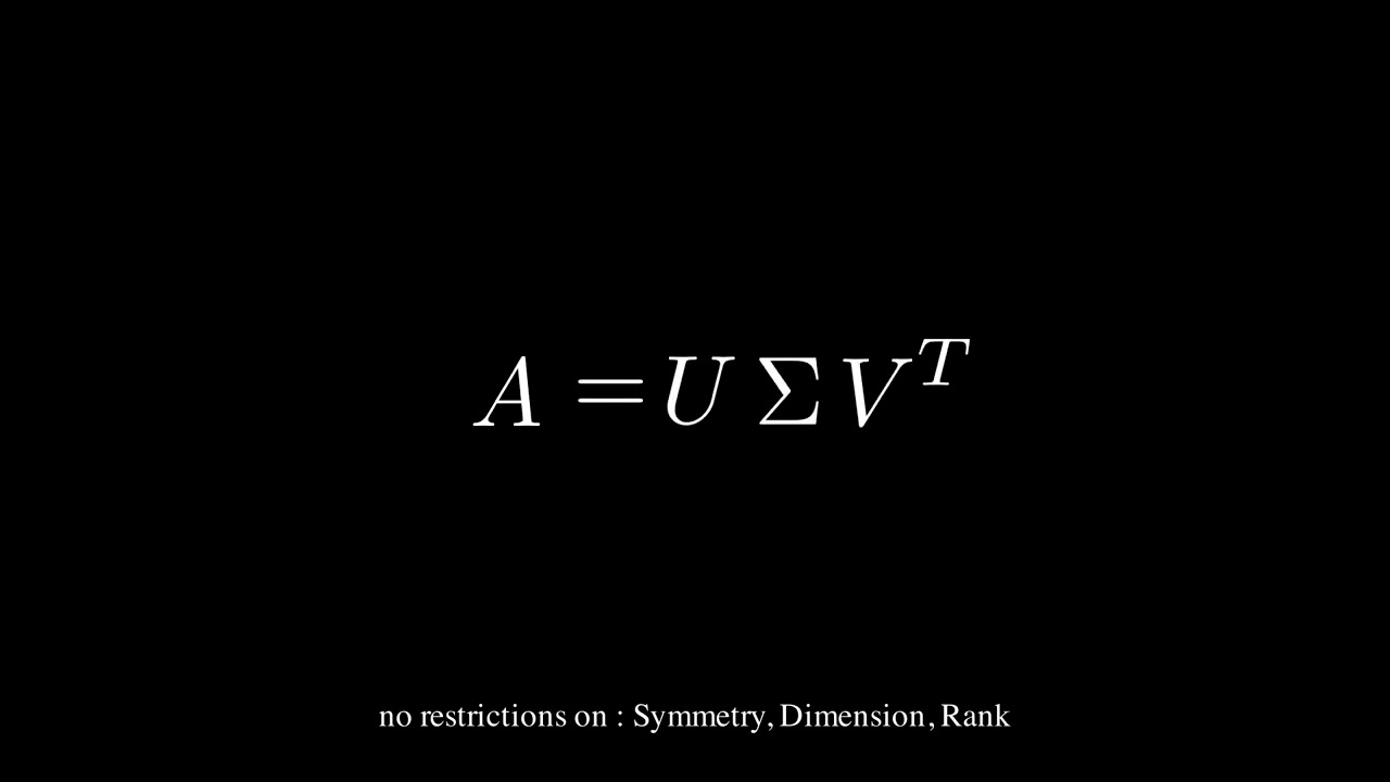
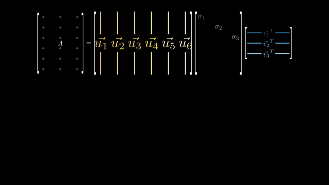
그때 분해되는 행렬이 바로 \(U, \Sigma, V\) 이렇게 세 개의 행렬인데요, 결론부터 말하자면 SVD를 할 경우 서로 직교하는 (Orthgonal) 특별한 벡터들로 이루어진 \(U, V\) 행렬을 얻을 수 있고 이 중 상위 몇개의 벡터들 (ex 8개) 만 사용해서 rank 1 의 행렬 8 개를 만듦으로써
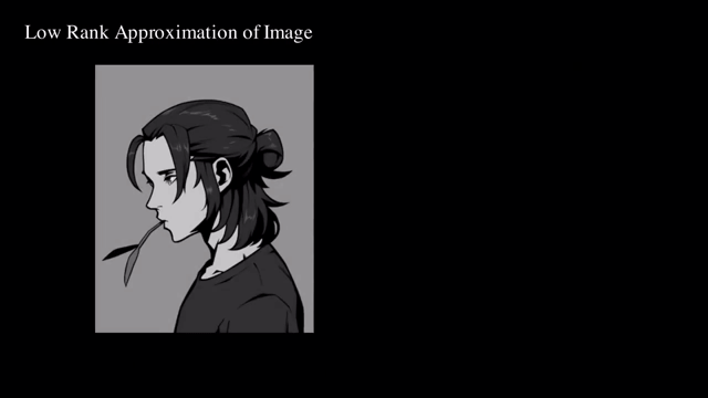
아래의 이미지를 나타내는 행렬을 원래 Rank보다 한참 낮은 Low Rank 로 근사하는, 즉 Low Rank Approximation (LRA) 를 수행함으로써 이미지를 압축하는 행위 등을 할 수 있습니다.
그렇다면 SVD 를 이루는 행렬은 어떤 특성을 가지고 있으며 왜 이것이 되는지 알아보겠습니다.
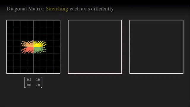
먼저 앞서 살펴본 몇 가지 중요한 행렬들을 remind해봅시다.
첫 번째는 단순하게 각 basis 축 을 기준으로 vector들을 늘려주는 것인데요, 바로 대각선 (diagonal) 부분에만 값이 있고 나머지 부분 (off-diagonal) 부분에는 0값으로 채워진 대각 행렬 (Diagonal Matrix) 로 이 행렬은 늘려주는 (Stretching) 행위를 하게 해줍니다.
그 다음으로는 basis vector 를 회전시키는 회전 행렬 (Rotation Matrix) 도 있었습니다.
이제 SVD 를 이해하기 위해서 몇가지 중요한 요소가 더 있는데요, 이는 다음과 같습니다.
첫째로 Dimension Eraser 과 Dimension Adder 입니다.
말 그대로 예를 들어 어떤 3차원 행렬에 Eraser를 쓰면 차원이 하나 사라지고 Adder를 쓰면 추가되는데요,
우리가 \((1,2), (1,2,0)\) 인 vector 를 갖고 있다고 생각해 봅시다.
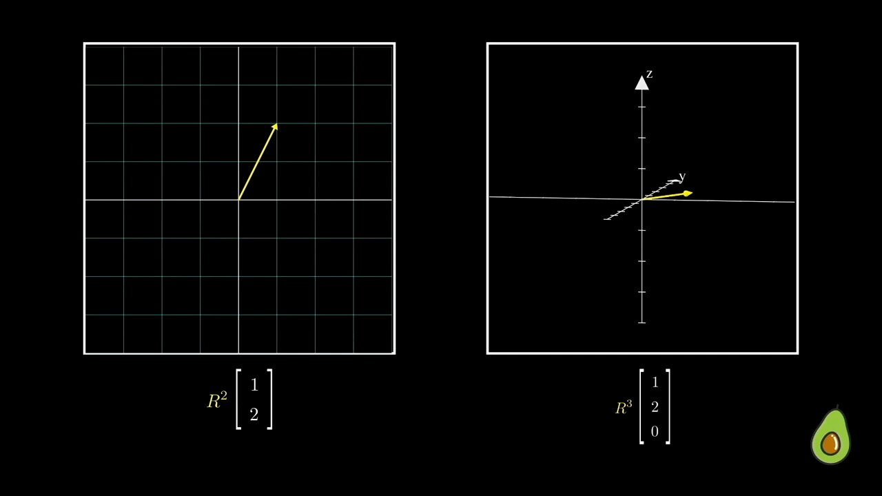
사실 이는 같은 벡터인데요, 다만 Dimension이 하나 추가된 것으로 볼 수 있습니다. 이 때 \((1,2,0)\) vector 를 2차원으로 바꿀 수가 있는데요, \(2 \times 3\) 차원의 행렬을 곱하면 됩니다.
하지만 이 때 아무거나 곱하면 안되고 원래 있던 basis 중 지우지 않을 차원의 basis는 건드리지 않게되면
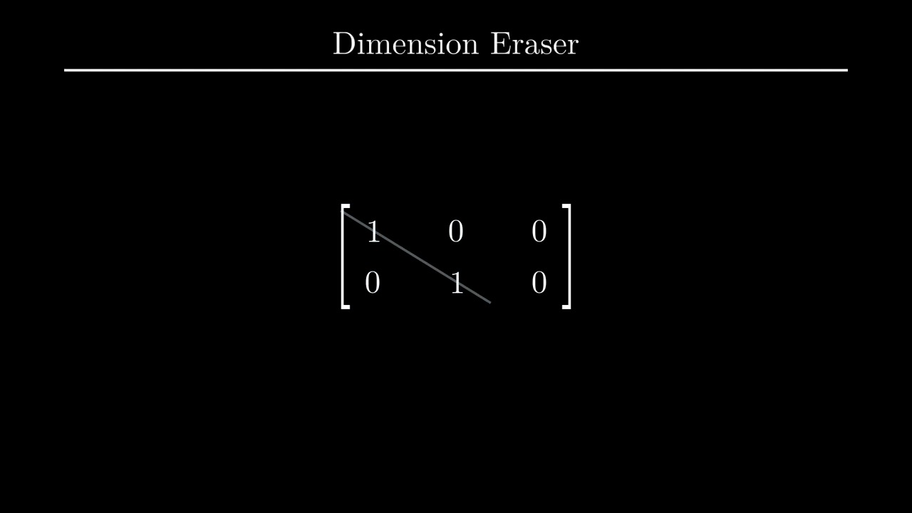
우리는 예를 들어 \(x,y,z\) 중 나머지는 건들지 않고 z 차원을 없애서 2차원으로 사영시킬 수 있습니다.
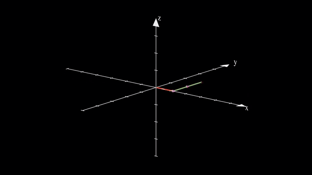
이는 같은 선상에 있는 모든 벡터들을 전부 같은 점으로 매핑시켜줍니다.
마찬가지로 vector 를 점으로 나타내듯 수많은 vector들을 뭉치를 하나의 object 로 생각해봐도 결과는 같습니다.
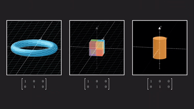
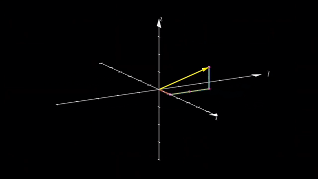
이렇게 차원을 없애는것과 반대로 더하는 것도 가능한데요, 예를 들어 2차원 행렬에 \(3 \times 2\) 행렬을 곱하면 3차원으로 보낼 수 있게 됩니다.
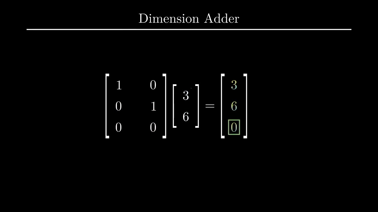
당연히 차원을 축소하고 늘릴때 대각성분이 1 (Identity Matrix) 일 필요는 없는데요, 만약 대각 성분에 1이 아닌 값이 있다면 Stretching 하는 결과를 가져올 겁니다.
이 전체 행렬은 근데 또 결국 Dimension Eraser + Stretching Matrix 의 조합으로 생각할 수 있겠습니다.
\[M_{m \times m}=P_{m \times m} D_{m \times m} P_{m \times m}^{-1}\] \[\begin{aligned} M & =P D P^{-1} \\ M(P) & =P D P^{-1}(P) \\ M P & =P D \end{aligned}\] \[\begin{aligned} & P=\left[a_1, a_2, \ldots a_m\right] \\ & D=\left[\begin{array}{cccc} \lambda_1 & 0 & \ldots & \ldots \\ 0 & \lambda_2 & 0 & \ldots \\ \vdots & \ldots & \ddots & \ldots \\ 0 & \ldots & 0 & \lambda_m \end{array}\right] \\ & P D=\left[\lambda_1 a_1, \lambda_2 a_2, \ldots \lambda_m a_m\right] \\ & \end{aligned}\]
하지만 모든 행렬에 대해 Diagonalization 을 수행할 수 있는건 (diagonlizable) 아닌데요, 즉 행렬 \(M\) 의 크기가 정사각형 \(n \times n\) 이어야 하며 Invertible 한 경우에만 이 연산이 가능합니다. 이를 해결하기 위해 Singular Vecotr Decomposition (SVD) 를 사용할 수 있는데요,
어떤 행렬 \(M\) 에 대해서 SVD 를 수행하면 아래와 같이 \(U,S,V\) 행렬을 얻을 수 있게 됩니다.
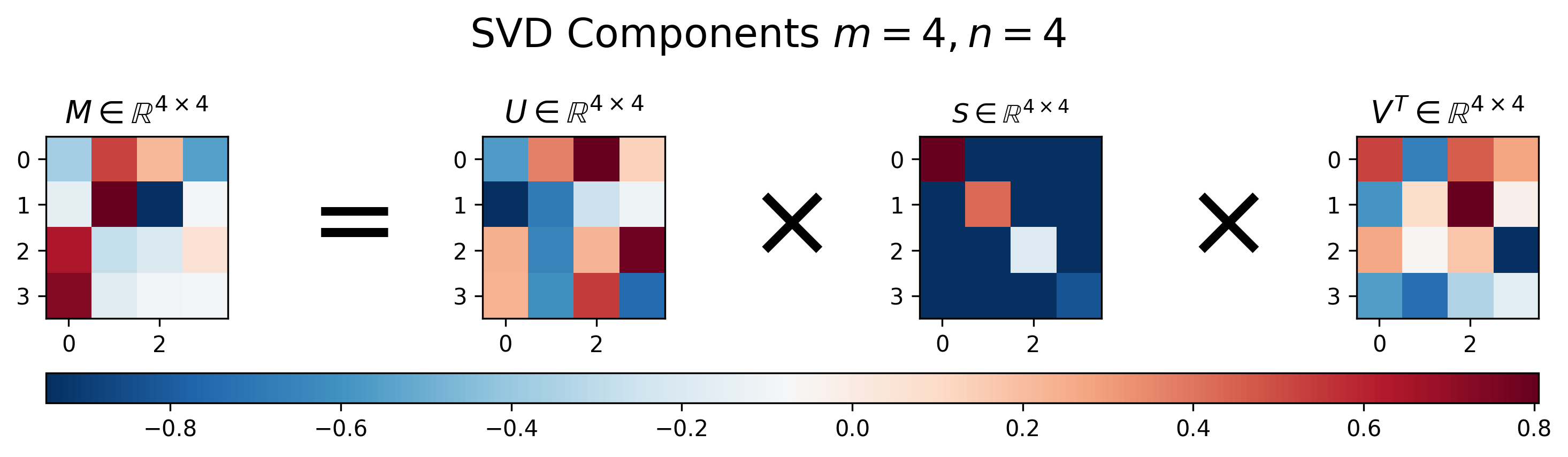
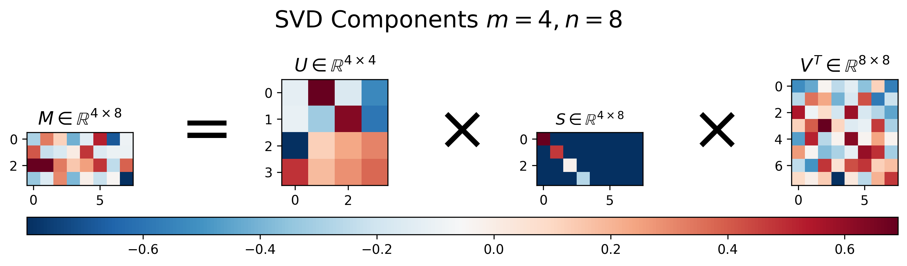
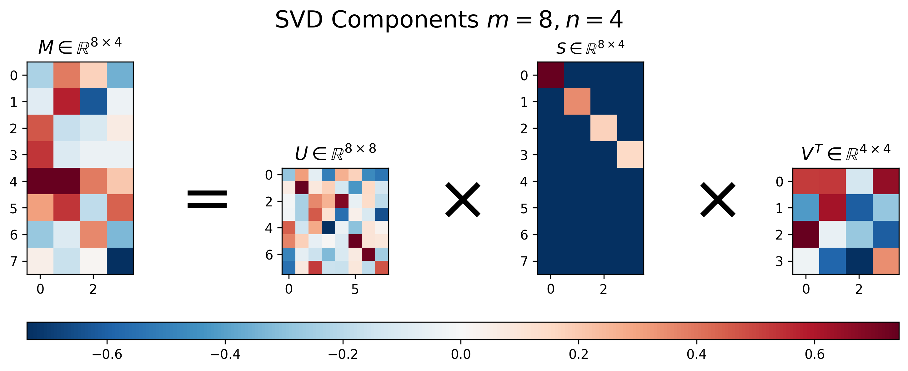 Fig. Vissualization of Results of SVD. Source From here
SVD 의 결과물을 보면 몇 가지 특이한 점을 알 수 있는데요, 바로
- U와 V의 모든 Column Vector 들은 크기 (norm) 가 1이다.
- U와 V의 Column Vector 들 간의 내적 (inner product) 을 취한 n x n Matrix 는 Identity Matrix 이다.
- U는 원본 행렬 M 의 \(MM^T\) 의 Eigenvector 를 가지고 있다.
- V는 원본 행렬 M 의 \(M^TM\) 의 Eigenvector 를 가지고 있다.
- S는 \(M^TM\) 와 \(MM^T\) 와 관련된 Eigenvalue 의 sqaure root 를 가지고 있다.
입니다.
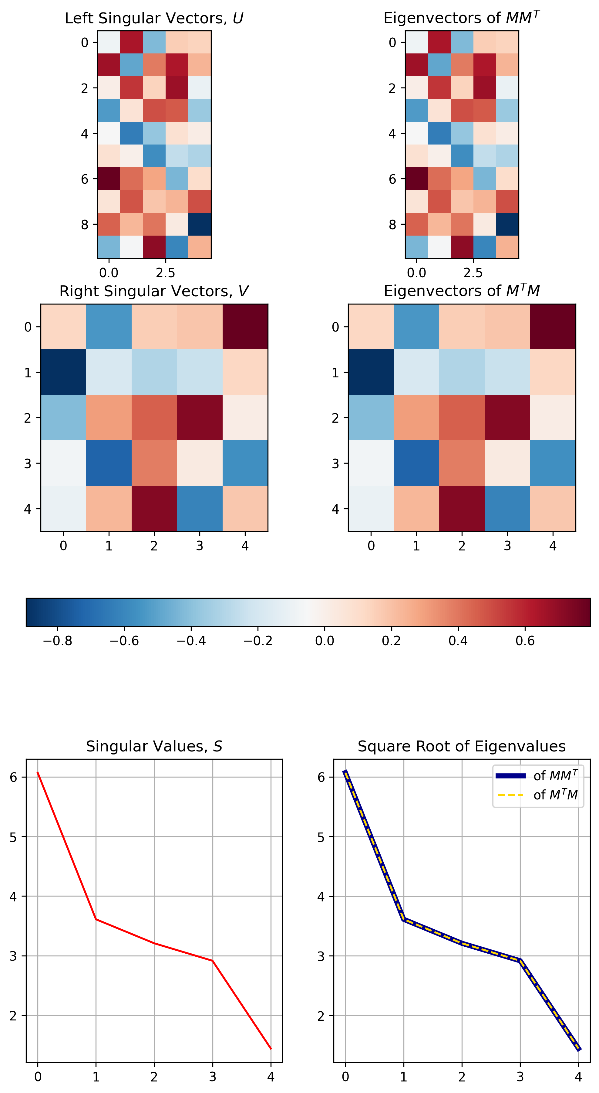 Fig. Eigenvalue Decomposition 과 SVD 의 관계. Source From here
SVD 를 잘 사용하면 여러 장점이 있지만 그 중에서 Low-Rank Matrix Approximation (LRA) 이라는 것이 가능해 집니다.
이는 \(US\) 와 \(V\) Matrix 들을 더 작은 크기의 Matrix 로 바꾸는 것인데요, SVD는 만약 Matrix 가 \(4 \times 4\) 일 경우 \(U \in \mathbb{R}^{4 \times 4}\), \(S \in \mathbb{R}^{4 \times 4}\), \(V \in \mathbb{R}^{4 \times 4}\) 를 얻을 수 있었죠,
하지만 우리는 이를 아래처럼 근사할 수 있습니다.
\[\begin{aligned} M & \approx U_k S_k V_k^T, \text{ where } k = 2 \\ & \approx \hat{M}_k \end{aligned}\]즉 우리는 \(U \in \mathbb{R}^{4 \times 2}\), \(S \in \mathbb{R}^{2 \times 2}\), \(V \in \mathbb{R}^{2 \times 4}\) 를 얻을 수 얻게 되는 건데요, 단순히 Matrix 가 Full Rank 일 때, 즉 Column 이 4일 때 Rank 가 4 인 경우에 이런 근사를 해버리면 좋지 않겠지만 우리가 만약 \(8 \times 8\) 크기의 행렬이지만 Rank 가 4 밖에 안되는 행렬을 가지고 있다면
![]() Fig. Matrix with Redundant Columns. Source From here
Fig. Matrix with Redundant Columns. Source From here
원래의 SVD를
\[\begin{aligned} M & =U S V^T \\ & =(U S) V^T \\ & =L R^T, \text { where } \\ L & =(U S), \text { and } \\ R & =V \end{aligned}\]근사해버려도 된다는 겁니다.
\[\begin{aligned} M & =L R^T \\ & \approx L_k R_k^T \\ & \approx \hat{M} \end{aligned}\]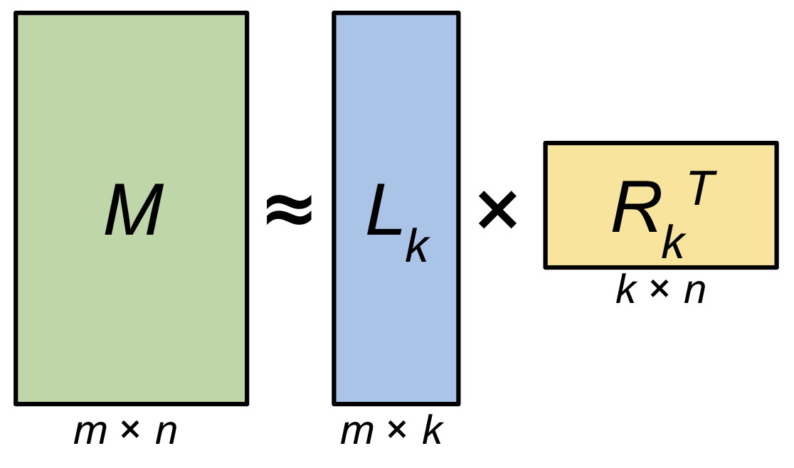 Fig. \(m \times n\) 크기의 Matrix \(M\) 을 \(m \times k\), \(k \times n\) 로 분해할 수 있다. 만약 \(k\) 가 데이터의 rank \(r\) 과 같다면 (\(r=k\)) Matrix \(M\) 은 완전히 Decomposition 으로부터 복원될 수 있고 \(k\)가 \(r\)보다 작으면, 즉 \(k<r\) 이면 근사된 Matrix, 즉 Low-Rank Approximated Matrix \(\hat{M}\) 을 얻을 수 있다.. Source From here
이렇게 근사를 해서 얻은 \(L, R (U,S,V)\) 를 사용해도 Redundant Column 이 포함되어 있는 행렬 \(\tilde{X}\) 를 복구하는데는 문제가 없다고 합니다.
![]() Fig. . Source From here
Fig. . Source From here
Matrix equals sum of rank-1 matrices
Principal Compenent Analysis (PCA) using SVD
Connection to the Fourier Transform
사실 SVD 라는 것은 신호 처리 (Digital Signal Processing; DSP) 의 퓨리에 변환 (Fourier Transform)과 비슷한 점이 많습니다.
Fourier Transform 은 어떤 Signal이 있을 때 이를 어떤 주기함수들의 결합으로 나타낼 수 있다는 아이디어에서 출발하는데요,
일반적으로 Cosine 함수와 Sin 함수를 무한히 결합해서 이를 만들어 냅니다.
SVD 라는 것은 어떤 행렬 A를 rank-1 짜리 행렬 여러개를 결합한 것으로 나타낼 수 있게해주고 Fourier Transform도 마찬가지로 서로 다른 주기를 가지고 있는 Sinusoidal Function 으로 결합할 수 있게 해줍니다.
반대로말하면 어떤 신호든, 행렬이든 나눠버릴 수 있게 해주는거죠.