Cheatsheet For "How To Scale"
10 Jul 2024< 목차 >
- tmp
- Refs
- Main Table
- Other Caveats for Training Large Transformers
- abc-parameterization symmetry
- Typical Init Std Values According To Width
- +Updated) An Ex-OpenAI Researcher Confirm OpenAI used muP
tmp
IMO, we should experiment in small scale regime to prove methods and find power law for example LR vs bsz. Howerver, small scale would not be enough because if we train model in larger tokens (or FLOPs), for example, LR sensitivity will be decreased and \(\sqrt{n}\) LR vs bsz scaling would not be correct in this regime. So my suggestion (from what I’ve observed so far) is,
-
- train small scale proxy model with enough steps for HP sweep or something
- e.g. 0.04B model / 131k batch tokens / 40000 steps / 5.24B tokens
- train small scale proxy model with enough steps for HP sweep or something
-
- compare new methods and former one in enough large scale
- e.g. SP vs muP in 1~2B models / 2M~4M batch tokens / 2T tokens
- compare new methods and former one in enough large scale
-
- run target configs
- e.g. muP (if its better than SP) in 8B~70B models / 8~15T tokens
- run target configs
(you should prove your hypothesis is right in 2nd step not 1st step)
Refs
- Key Papers
- Summaries
Main Table
This table is primarily derived from Tensor Program (TP) 4 and 5
| hparams | embedding | hidden | residual_out | unembedding (readout) |
|---|---|---|---|---|
| init_std (b) | \(\sigma_\text{embed}\) | \(\sigma_\text{hidden} \cdot (\color{red}{\tilde{n}})^{-0.5}\) | \(\sigma_\text{res-out} \cdot (\color{red}{\tilde{n}})^{-0.5} \cdot (2 n_\text{layers})^{-0.5}\) | \(\sigma_\text{un-embed}\) |
| multiplier (a) | \(\alpha_{\text{embed}} \cdot 1\) | \(\alpha_{\text{hidden}} \cdot 1\) | \(\alpha_{\text{res-out}} \cdot 1\) | \(\alpha_{\text{un-embed}} \cdot (\color{red}{\tilde{n}})^{-1}\) |
| adamw lr (c) | \(\eta_{\text{embed}} \cdot (\color{green}{\tilde{b}})^{0.5} \cdot {(\color{blue}{\tilde{d}})^{\alpha_{\text{data}}}}\) | \(\eta_{\text{hidden}} \cdot (\color{red}{\tilde{n}})^{-1} \cdot (\color{green}{\tilde{b}})^{0.5} \cdot {(\color{blue}{\tilde{d}})^{\alpha_{\text{data}}}}\) | \(\eta_{\text{res-out}} \cdot (\color{red}{\tilde{n}})^{-1} \cdot (\color{green}{\tilde{b}})^{0.5} {(\color{blue}{\tilde{d}})^{\alpha_{\text{data}}}}\) | \(\eta_{\text{un-embed}} \cdot (\color{green}{\tilde{b}})^{0.5} {(\color{blue}{\tilde{d}})^{\alpha_{\text{data}}}}\) |
| adamw moment | \((1-\color{green}{\tilde{b}}(1-\beta_1),\\1-\color{green}{\tilde{b}}(1-\beta_2))\) | \((1-\color{green}{\tilde{b}}(1-\beta_1),\\1-\color{green}{\tilde{b}}(1-\beta_2))\) | \((1-\color{green}{\tilde{b}}(1-\beta_1),\\1-\color{green}{\tilde{b}}(1-\beta_2))\) | \((1-\color{green}{\tilde{b}}(1-\beta_1),\\1-\color{green}{\tilde{b}}(1-\beta_2))\) |
| adamw epsilon | \(\epsilon \cdot (\color{green}{\tilde{b}})^{-0.5}\) | \(\epsilon \cdot (\color{green}{\tilde{b}})^{-0.5}\) | \(\epsilon \cdot (\color{green}{\tilde{b}})^{-0.5}\) | \(\epsilon \cdot (\color{green}{\tilde{b}})^{-0.5}\) |
| adamw weight_decay | \(\lambda\) | \(\lambda\) | \(\lambda\) | \(\lambda\) |
 Fig. Table 8 from TP-V
 Fig. Table 2 from unit-muP. it reflects TP-VI too
Key Intuition for muP (Maximal Update Parameterization)
- What we want is every (pre-)activations has constant scale (\(\Theta(1)\)) at any time in training
- so we have to properly scale init std of params, learning rate and multiplier to ensure \(W_{t+1} x' = (W_{t} + \eta \Delta W_{t})x' = W_t x' + n \eta g_t \frac{(x^T x')}{n}\) has constant scale. here \(\frac{(x^T x')}{n}\) return deterministic scalar by Law of Large Numbers (LLN)
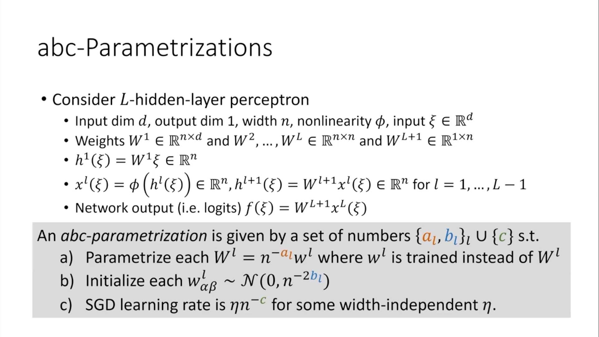
- TP defines abc-parameterization
a: we parameterize each weight parameters as \(W^{l} = n^{-a_l} w^l\) for actual trainable param \(w^l\)b: we init each \(w^l \sim \mathcal{N}(0, n^{-2b_l})\)c: the SGD learning rate is \(\eta n^{-c}\) for some width-independent \(\eta\)
 Fig.
Fig.
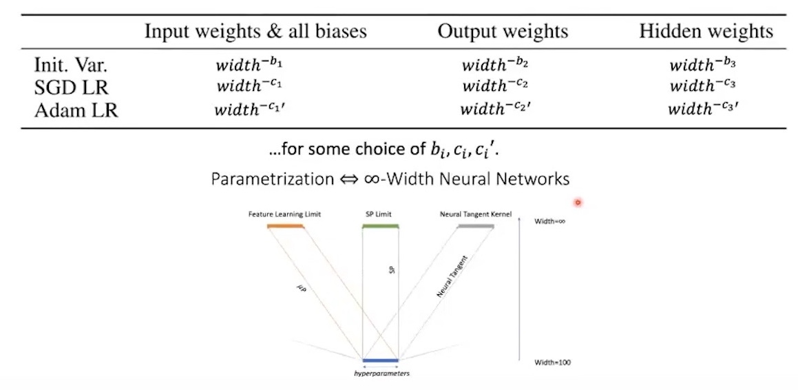
- Main Question: “How to correctly set
per layers a, b, cto make layers’ activation do not blow up (training stability) and ensure every layers to be trained equally? (maximal feature learning) as Neural Network (NN)’s width goes to infinity?”
 Fig.
Fig.
- The mathematically derived answer to this question is TP 4, 5 and it ensure maximal feature learning and training stability for inifinite width NN
 Fig. Maximal Update Parameterization Table
Notation and Explanation
width: width means hidden size (or head dimension) of NN (Transformer). For small scale proxy (base) models, shape of specific layer’s weight parameter is \(W_l \in \mathbb{R}^{ {\text{fan-in}}_{\text{base}} \times {\text{fan-in}}_{\text{base}} }\). In TP-5 paper, Table 3, 8, 9 describe parameterizations usingfan_inandfan_outwhere they are input feature dimension and output feature dimension each. however in this table, \(\tilde{n}=\text{fan-in} \cdot \frac{1}{\text{fan-in}_\text{base}}\) and if \(\text{fan-in}_\text{base} = 1\), it recovers Table 8. and if \(\sigma = 1/\sqrt{1024} \approx 0.31\), ini_std become \(1/\text{fan-in}\)- for example, \(\color{red}{\tilde{n}=100}\)
multiplier- Note that there is 2 multiplier, one is for scaling and another is for hparam for example. for example, embedding outputs are like
x = hparam_multiplier * width_scaling_multiplier * embedding_layer(x)where multiplier does not scale as the width increases andhparam_multiplieris hparam like lr. - We can set tunable multiplier, \(\alpha_{\text{embed}}=10\) (based on the results of various papers using muP) and multiper for scaling by 1.
- While i just use same sigma and lr for all parameters, one can set per layer values for every per layer parameterization (init_std, lr or hparam_multiplier)
- Note that there is 2 multiplier, one is for scaling and another is for hparam for example. for example, embedding outputs are like
LR scaling according to batch size: In general case, lr decrease and batch size increase as model size grows. however when muP is applied, optimal lr is transferred (for sufficiently large batch size). but muP doesnt gaurantee optimal scaling where if we want to increase batch size by \(n\) times, we should scale LR \(\sqrt{n}\) as well. we define \(\tilde{b} = \text{bsz} / \text{bsz}_{\text{base}}\)- for example, \(\color{green}{\tilde{b} = 8}\) (4e6 (4M) for target model and 500e3 (500k) for small scale model)
- LR scaling should be \(\eta \cdot (\color{green}{\tilde{b}})^{0.5}\) (it is not optimal but well-known heuristic)
- Note that, we should consider critical batch size where if batch size is greater than ‘some point’, it does not decrease training time efficiently as the number of GPU devices grows. Therefore,
we should not set the largest batch size we can with the total GPU resources we currently have available but proper batch size as long as it doesn't damage the MFUs.
attention logit scaling- Unless you have plan to scale depth, scale factor of Scaled Dot Product Attention (SDPA), scaling factor is \(d_\text{head}\), not \(\sqrt{d_\text{head}}\) for \(QK^T/scale\) because \(q,k\) will be correlated after training start so it should be scaled according to LLN (attention operator also have attn_multipler, but we set this 1.0 typically)
dataset size: Typically small scale proxy models consume much smaller tokens e.g. 1/100 of target processed tokens . we define \(\color{blue}{\tilde{d}} = (\frac{d_{\text{large}}}{d_{\text{small}}})\) and \(\alpha_\text{data}\), whered_large/d_smallis data fraction between small scale proxy and target size models and \(\alpha_{\text{data}}\) is scaling exponents. in TP-V, they fixed training steps and transfer LR, so in realistic setting where dataset size, D is scaled too, it’s not optimal.- for example, if \(d_{\text{large}}=8T\), \(d_{\text{small}}=80B\), then \(\color{blue}{\tilde{d}=100}\). but how can we get \(\alpha_{\text{data}}\)? to my best knowledge, there is no theoritical equation. this paper said \(-0.12\) is good for chinchilla scaling rule where N and D is equally scaled when C is increased and N is quadratic to width \(n\). so it returns \(n^{-1} \cdot n^{2 \cdot -0.12}=n^{-1.24}\).
- What HPs should we search?
- we want to saerch HP in small scale and then transfer, but what HPs should we search? there are many HPs, lr, init_std and so on (\(\eta_{\text{embed}}, \cdots, \sigma_\text{embed}, \cdots\)) but typically global LRs and are same for all parameters (but it’s probably not optimal) and so is init std.
- Zero variance init
- it is recommended to use zero init to remove discrepency between small and target scale models (see TP-V paper)
- q proj
- residual out layer
- redaout (lm_head)
- it is recommended to use zero init to remove discrepency between small and target scale models (see TP-V paper)
- Optimizer HPs
- Use \((\beta_1, \beta_2)=(0.9, 0.95)\) and \(\epsilon=1\text{e-}8\) which is typical values for LLM
- however if you want scale batch size as cumpute budget grows, there is an opinion suggesting larger beta for small batches (small batch == small LR)
- For weight decay, \(\lambda\), set 1e-1 for pytorch default, and 1e-4 for
tensorflow adamwortruly decoupled adamw, because pytorch default multiply wd value by lr, it should be larger.- you can train small scales withoud weight_decay and introduce it when you train target model
- Recently proposed papers related to muP claims truly decoupled adamw fixes HP transfer stability
- it’s easy to implement by setting
weight_decayasweight_decay / group['lr']
- Use \((\beta_1, \beta_2)=(0.9, 0.95)\) and \(\epsilon=1\text{e-}8\) which is typical values for LLM
Other Caveats for Training Large Transformers
- Track Machine FLOPs Utilization (MFU)
- MFU means “how many FLOPs do you utilize in a second”. you should track MFU and if it’s lower than 50% (in general case e.g. 128~256 GPUs), there might be bottleneck somewhere for example because the degree of tensor parallelism (TP) is too high or gradient checkpoints are applied too often, and so on…
- but if parallelism degree is excessively large (e.g. llama-3 trained 405B model with 8192~16384 GPUs), it’s hard to achieve high MFU.
- MFU means “how many FLOPs do you utilize in a second”. you should track MFU and if it’s lower than 50% (in general case e.g. 128~256 GPUs), there might be bottleneck somewhere for example because the degree of tensor parallelism (TP) is too high or gradient checkpoints are applied too often, and so on…
- Use
bfloat16rather thanfloat16- It’s dynamic range is same as float32 and does not require dynamic loss scale (no overhead)
- Monitor logits
- two logits (quantities before softmax operation) contribute training instability
- attention logits: use qk-layernorm but it might require additional computation
- output logits: use z-loss (also require additional computational cost)
- Recently, Gemma-2 proposed attention logit soft-capping for stability (Grok also use same strategy)
- two logits (quantities before softmax operation) contribute training instability
Remove Bias termin Linear layers- Most of frontier LLMs has no bias term in every Linear layers but recently proposed SOTA LLM (30/06/24), Qwen2 include bias terms for better generlization in long context
- Doubt Optimizer HPs
- Set gradient clipping factor as 1.0
- Be careful of Adam’s EMA factor, \(\beta_1, \beta_2\) and \(\epsilon\)
- nn.layernorm vs RMSNorm
- TBC
abc-parameterization symmetry
from torch import manual_seed, nn, optim, randn
manual_seed(1234)

### Uncomment one of these lines -> in both cases y2 comes out the same!
lr = 1; mult = 1e-3; init_std = 1 / mult;
# lr = 1e-3; mult = 1; init_std = 1

l = nn.Linear(1024, 2048, bias=False)
nn.init.normal_(l.weight, std=init_std)
model = lambda x: l(x) * mult
opt = optim.Adam(l.parameters(), lr=lr, eps=0)

x = randn(512, 1024).requires_grad_()
y1 = model(x).mean()
print(y1)
y1.backward(); opt.step()
y2 = model(x).mean()
print(y2)  # Comes out the same, regardless of LR
Source from Charlie Blake
Typical Init Std Values According To Width
It is noteworthy that some opensource frameworks model config set std=0.02 that is hardcoded value for GPT-2 (maximum 1.5B scale).
If you try to train 30B, 60B, … model with this std without considering increased hidden size,
welcome to hell.
>>> for d in range(256,8192+256,256):
...     print(f"d_model (width): {d}, 1/sqrt(width): {1/math.sqrt(d)}")
...
d_model (width): 256, 1/sqrt(width): 0.0625
d_model (width): 512, 1/sqrt(width): 0.044194173824159216
d_model (width): 768, 1/sqrt(width): 0.036084391824351615
d_model (width): 1024, 1/sqrt(width): 0.03125
d_model (width): 1280, 1/sqrt(width): 0.02795084971874737
d_model (width): 1536, 1/sqrt(width): 0.025515518153991442
d_model (width): 1792, 1/sqrt(width): 0.0236227795630767
d_model (width): 2048, 1/sqrt(width): 0.022097086912079608
d_model (width): 2304, 1/sqrt(width): 0.020833333333333332
d_model (width): 2560, 1/sqrt(width): 0.01976423537605237
d_model (width): 2816, 1/sqrt(width): 0.018844459036110227
d_model (width): 3072, 1/sqrt(width): 0.018042195912175808
d_model (width): 3328, 1/sqrt(width): 0.01733438113203841
d_model (width): 3584, 1/sqrt(width): 0.016703827619526525
d_model (width): 3840, 1/sqrt(width): 0.01613743060919757
d_model (width): 4096, 1/sqrt(width): 0.015625
d_model (width): 4352, 1/sqrt(width): 0.01515847656477081
d_model (width): 4608, 1/sqrt(width): 0.014731391274719742
d_model (width): 4864, 1/sqrt(width): 0.014338483366910109
d_model (width): 5120, 1/sqrt(width): 0.013975424859373685
d_model (width): 5376, 1/sqrt(width): 0.013638618139749524
d_model (width): 5632, 1/sqrt(width): 0.013325044772225651
d_model (width): 5888, 1/sqrt(width): 0.013032150878567173
d_model (width): 6144, 1/sqrt(width): 0.012757759076995721
d_model (width): 6400, 1/sqrt(width): 0.0125
d_model (width): 6656, 1/sqrt(width): 0.012257258446136503
d_model (width): 6912, 1/sqrt(width): 0.012028130608117204
d_model (width): 7168, 1/sqrt(width): 0.01181138978153835
d_model (width): 7424, 1/sqrt(width): 0.011605958636065741
d_model (width): 7680, 1/sqrt(width): 0.01141088661469096
d_model (width): 7936, 1/sqrt(width): 0.011225331376673432
d_model (width): 8192, 1/sqrt(width): 0.011048543456039804
+Updated) An Ex-OpenAI Researcher Confirm OpenAI used muP
Andrew Carr confirmed.
 Fig.
Fig.
 Fig.
Fig.