Rethinking Self Attention with Kernel and Rank (Towards More Efficient and Effective Transformer)
14 Jan 2023< 목차 >
- Motivation
- Performer (2020)
- Connection to Linformer
- Pytorch Implementation
- References
Motivation
이번 Post 는 Rethinking Attention with Performers 라는 논문의 내용을 기반으로 작성되었습니다. 이 논문의 motivation 은 "Transformer 의 Attention 연산을 잘 분석해서 모델의 Space Complexity 와 Time Compelxtiy를 줄여보자" 입니다.
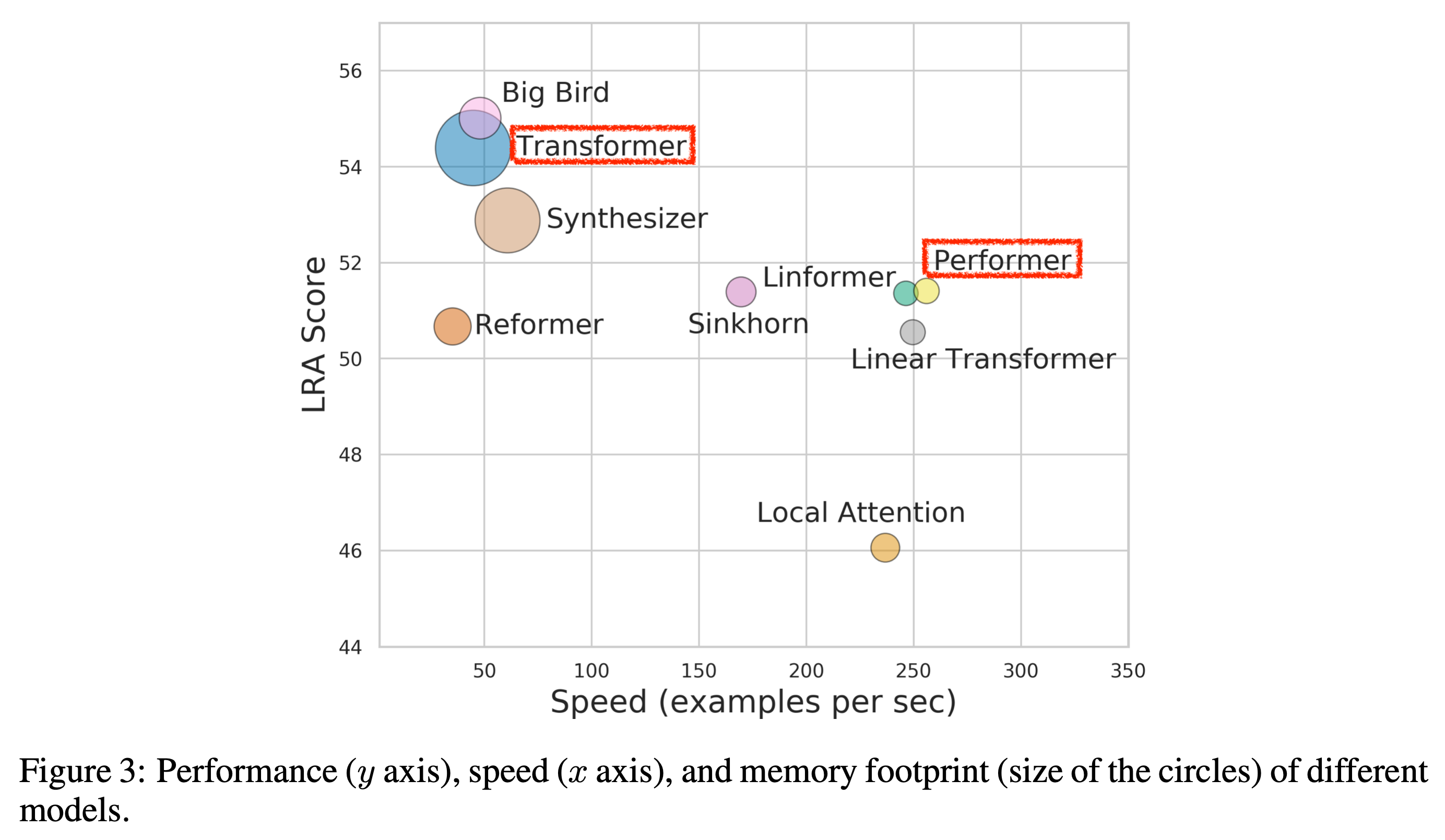 Fig. Long Range Arena Benchmark Score. Performer 는 Transformer 와 비교했을 때 성능면에서 조금 손해가 있으나 Long Range Sequence 에 대해 더 적은 메모리가 필요하며 (원이 작을수록 적은 메모리가 필요), 속도는 5배 이상 빠르다.
Performer (2020)
Standard Attention Module
Vanilla Tranformer 의 Scaled Dot Product Self-Attention (SA) Mechanism 을 Recap 해 봅시다.
이는 아래와 같은 수식을 따르는데요,
Layer 의 Input Token 을 Query (Q), Key (K), Value (V) 로 변환한 뒤 \(Q^TK\) 를 통해 Token 간의 Relationship 을 계산하고 V 를 곱해 Token 들간의 정보를 서로 Mixing 해줍니다.
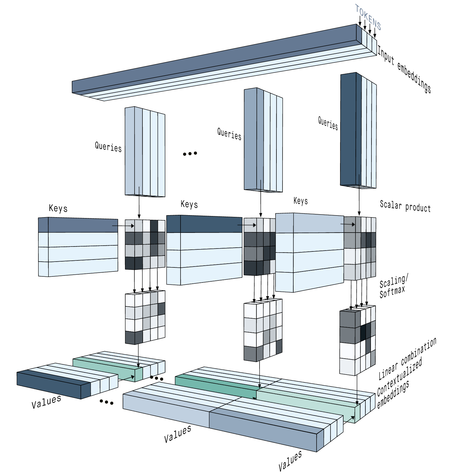 Fig. Attention From Inputs to Outputs (Cross-Attention). Source from peltarion’s post
이 때의 시간 복잡도 (Time Compleixty) 와 공간 복잡도 (Space Complexity) 는 다음과 같은데
- Space Complexity : \(O(L^2 + Ld)\)
- Time Complexity : \(O(L^2d)\)
이는 \(Q,K,V\) 가 각각 \(\mathbb{R}^{L \times d}\) 일 때의 복잡도이며, 이 때 \(L\) 은 Sequence 의 길이 (Token의 개수) 이고 \(d\) 는 각 Token Vector 들의 크기 입니다.
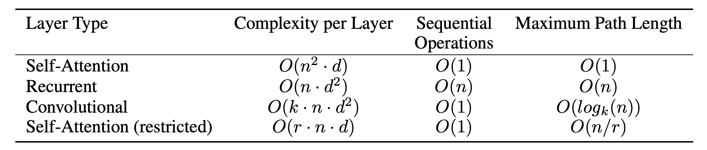 Fig. Self Attention Mechanism’s Time Complexity
근데 왜 복잡도가 이렇게 Sequence 길이의 제곱 (Quadratic) 이 되는 걸까요?
맨 처음 입력 벡터들을 Q, K, V 로 각각 변환해 주는 것은 Linear Transformation 입니다. Q, K, V Projection 이 원래 차원을 유지하는 변환이라고 생각할 경우 \(d \times d\) 차원의 행렬과 \(L \times d\) 차원의 Input Matrix 를 곱하는 것이므로 \(O(n d^2)\) 의 연산량이 듭니다. 하지만 일반적으로 이 연산은 Self Attention 의 복잡도를 구할때 고려되지 않는다고 합니다. 이미 되어있다고 보고 Self-Attention 에 대해서만 계산하는거죠.
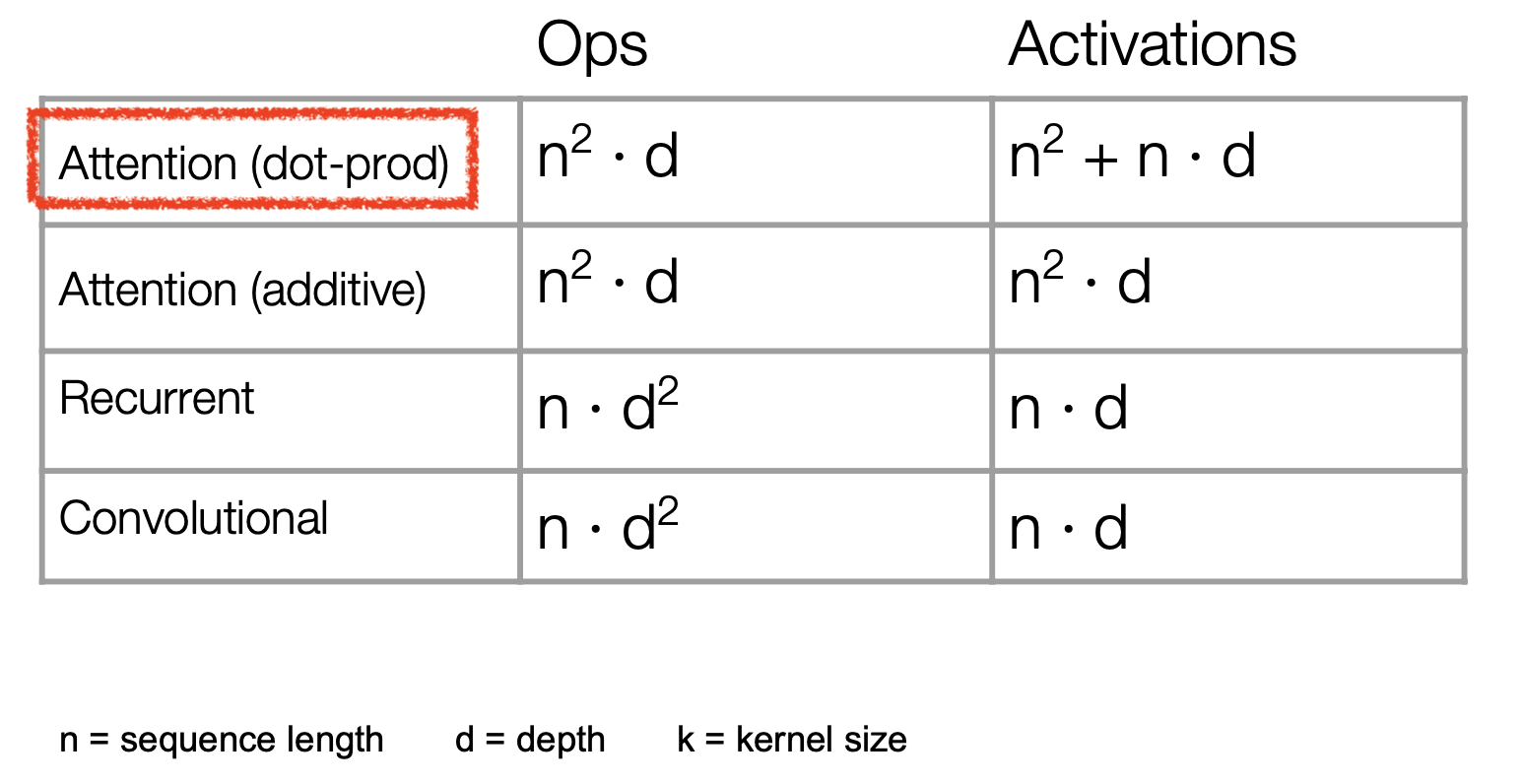 Fig. Scaled Dot Product Self Attention. Source from link
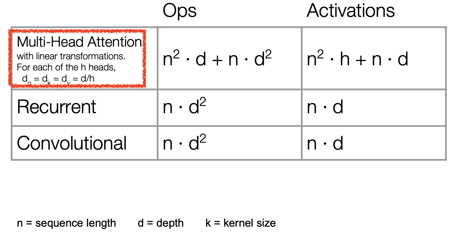 Fig. Scaled Dot Product Multi Head Self Attention with Q, K, V Projection. Source from link
그다음으로는 \(Q^T K\) 인 행렬 곱을 해야되는데요, 어떤 \(n \times m\) 크기의 \(A\) 와 \(m \times p\) 크기의 \(B\) 행렬들이 있을 때 두 행렬의 곱인 \(C=AB\) 는 \(n \times p\) 크기가 되며
\[C_{ij} = \sum_{k=1}^{n} A_{ik} B_{kj}\]이 때 연산은 아래와 같이 단순하게 구현할 수 있습니다.
Input: matrices A and B
Let C be a new matrix of the appropriate size
For i from 1 to n:
    For j from 1 to p:
        Let sum = 0
        For k from 1 to m:
            Set sum ← sum + Aik × Bkj
        Set Cij ← sum
Return C
즉 \(1 \times m\) 크기의 벡터들 p개 끼리 내적 (inner product; dot product) 하는 것을 n 번 반복 하는게 되는 겁니다. 이때의 time complexity 는 \(O(nmp)\) 가 되는데 만일 \(A,B\) 가 모두 \(n \times n\) 이라면 \(O(n^3)\) 가 됩니다. 그러니까 Self-Attention 의 경우 \(L \times d\) 인 두 행렬 \(Q,K\) 에 대해 \(Q^T K\) 연산을 취하므로 \(O(LdL) = O(L^2d)\) 만큼의 시간 복잡도가 드는 것입니다.
\[\frac{Q K^T}{\sqrt{d_k}}\]여기에 \(\sqrt{d_k}\) 로 행렬을 Normalize 해주고 Row-wise 로 Softmax 연산을 취해주는 것은 row vector 를 순회해서 sum of exponential 을 해줘야 하는 것을 Token 갯수만큼 반복해야 하기 때문에 \(O(Ld)\) 가 될것이고,
\[\operatorname{softmax}\left(\frac{Q K^T}{\sqrt{d_k}}\right)\]마지막으로 \(V\) 를 곱하는것 또한 \(L \times L\) 행렬과 \(L \times d\) 간의 행렬곱이기 때문에 \(O(L^2 d)\) 만큼의 연산이 들기 때문에 최종적으로 \(O(2L^2d + Ld) = O(L^2d)\) 가 되는 것입니다.
Scaled Dot Product Self Attention in Performer Paper
Scaled Dot Product Self Attention 을 Performer 논문에서는 아래와 같이 표현하는데요,
\[\operatorname{Att}_{\leftrightarrow}(\mathbf{Q}, \mathbf{K}, \mathbf{V})=\mathbf{D}^{-1} \mathbf{A V}, \quad \mathbf{A}=\exp \left(\mathbf{Q} \mathbf{K}^{\top} / \sqrt{d}\right), \quad \mathbf{D}=\operatorname{diag}\left(\mathbf{A} \mathbf{1}_L\right)\] \[\operatorname{Att}_{\rightarrow}(\mathbf{Q}, \mathbf{K}, \mathbf{V})=\widetilde{\mathbf{D}}^{-1} \widetilde{\mathbf{A}} \mathbf{V}, \quad \widetilde{\mathbf{A}}=\operatorname{tril}(\mathbf{A}), \quad \widetilde{\mathbf{D}}=\operatorname{diag}\left(\tilde{\mathbf{A}} \mathbf{1}_L\right)\]첫 번째는 일반적인 Self Attention 으로 Encoder 에서 수행되는 것이며, 두 번째는 Decoder 에서 수행되는 Unidirectional Self Attention 입니다.
Notation 이 좀 헷갈리실 수 있는데요, Q, K, V 는 원 논문의 \(L \times d\) 차원의 Query, Key, Value 이며 \(\mathbb{1}_L\) 은 모든 element 를 1로 갖는 길이가 L 인 vector 입니다.
먼저 \(Q,K\) 를 이용해 \(L \times L\) 차원의 Attention Score Matrix \(A\) 를 만들 수 있죠, 여기서 우리가 더 해줘야 하는것은
- 입력 벡터의 크기로 Scaling 해주는 것
- Softmax 함수로 Normalization 해줄 것
- V 를 곱해 최종적인 Context Vector 들을 만들 것
입니다.
Scailing 은 그냥 해주면 되고요,
\[\mathbf{A}=\exp \left(\mathbf{Q} \mathbf{K}^{\top} / \sqrt{d}\right)\]Softmax 를 그냥 해줄수도 있지만 논문에서는 \(\mathbb{1}_L\) 를 이용해서 이를 처리합니다. 이를 위해 먼저 아래의 연산을 해주는데
\[\mathbf{D}=\operatorname{diag}\left(\mathbf{A} \mathbf{1}_L\right)\]행렬 \(A\) 에 \(L \times 1\) 짜리 \(\mathbb{1}_L\) 를 곱해주면 row-wise 로 모두 더하는 연산을 해주게 됩니다.
\[\mathbf{A} \mathbf{1}_L = \begin{bmatrix} A_{11} & A_{12} & \cdots & A_{1L} \\ \vdots & \ddots & \cdots & \cdots \\ A_{L1} & A_{L2} & \cdots & A_{LL} \\ \end{bmatrix} \begin{bmatrix} 1 \\ \vdots \\ 1 \\ \end{bmatrix} = \begin{bmatrix} \sum_{i=1}^{L} A_{1i} \\ \vdots \\ \sum_{i=1}^{L} A_{Li} \\ \end{bmatrix}\]처음에 정의할 때 \(A\) matrix 자체를 \(QK^T\) 행렬에 exponential 연산까지 한 것으로 정의 했기 때문에 이 연산 자체가 Softmax 의 분모가 되고,
\[Softmax (z) = \frac{ \exp (z_i) }{ \sum_{i=1}^{k}{ \exp (z_i) } } \text{ , where } z \in \mathbb{R}^{k}\]이 \(\mathbf{A} \mathbf{1}_L\) vector를 다시 \(L \times L\) 행렬로 만들기 위해 어떤 input vector 를 diagnoal 로 갖는 행렬로 바꿔주는 새로운 연산자 \(diag\) 를 정의한 뒤
\[\mathbf{D}=\operatorname{diag}\left(\mathbf{A} \mathbf{1}_L\right) = \begin{bmatrix} \sum_{i=1}^{L} A_{1i} & 0 & \cdots & 0 \\ 0 & \sum_{i=1}^{L} A_{2i} & 0 & 0 \\ \vdots & 0 & \ddots & \vdots \\ 0 & 0 & \cdots & \sum_{i=1}^{L} A_{Li} \\ \end{bmatrix}\]이 \(D\) 행렬의 역행렬을 곱해주면
\[\mathbf{D^{-1}} = \begin{bmatrix} \frac{1}{\sum_{i=1}^{L} A_{1i}} & 0 & \cdots & 0 \\ 0 & \frac{1}{\sum_{i=1}^{L} A_{2i}} & 0 & 0 \\ \vdots & 0 & \ddots & \vdots \\ 0 & 0 & \cdots & \frac{1}{\sum_{i=1}^{L} A_{Li}} \\ \end{bmatrix}\]사실상 \(Softmax (\frac{QK^T}{\sqrt{d}})\) 연산을 한 것이나 다름 없고,
\[\mathbf{D}^{-1} \mathbf{A}\]마지막으로 \(V\) 를 곱해주면 Scaled Dot Proudct Self Attention 을 행렬 곱으로만 표현할 수 있게 됩니다.
\[\operatorname{Att}_{\leftrightarrow}(\mathbf{Q}, \mathbf{K}, \mathbf{V})=\mathbf{D}^{-1} \mathbf{A V}, \quad \mathbf{A}=\exp \left(\mathbf{Q} \mathbf{K}^{\top} / \sqrt{d}\right), \quad \mathbf{D}=\operatorname{diag}\left(\mathbf{A} \mathbf{1}_L\right)\]이를 어떤 행렬의 Diagonal 을 포함한 Lower Triangle part 만을 취하는 연산자 \(tril(\cdot)\) 을 정의해서 아래처럼 쓰면
\[\operatorname{Att}_{\rightarrow}(\mathbf{Q}, \mathbf{K}, \mathbf{V})=\widetilde{\mathbf{D}}^{-1} \widetilde{\mathbf{A}} \mathbf{V}, \quad \widetilde{\mathbf{A}}=\operatorname{tril}(\mathbf{A}), \quad \widetilde{\mathbf{D}}=\operatorname{diag}\left(\tilde{\mathbf{A}} \mathbf{1}_L\right)\]Transformer Decoder 모듈의 Unidirectional Self Attention 까지 표현할 수 있게 되었습니다.
왜 이렇게까지 해야하느냐? 이는 곧 논문을 살펴보면서 알게 될겁니다.
Standard Sparsification Techniques and Limitations
Self-Attention 의 한계점은 Sequence 의 길이 \(L\)이 늘어나면 늘어날수록 필요한 Memory 와 Latency 가 늘어난다는 데 있습니다. 이를 해결하기 위해서 다양한 Self Attention 의 변형체들이 매 해 수없이 등장해왔는데 그 중 대표적인 논문들로 아래와 같은 논문들이 있었습니다.
 Fig.
Fig.
(1) They require efficient sparse-matrix multiplication operations, which are not available on all accelerators
(2) they usually do not provide rigorous theoretical guarantees for their representation power
(3) they are optimized primarily for Transformer models and generative pre-training
(4) they usually stack more attention layers to compensate for sparse representations, making them difficult to use with other pre-trained models, thus requiring retraining and significant energy consumption.
In addition to these shortcomings, sparse attention mechanisms are often still not sufficient to address the full range of problems to which regular attention methods are applied, such as Pointer Networks.
There are also some operations that cannot be sparsified, such as the commonly used softmax operation, which normalizes similarity scores in the attention mechanism and is used heavily in industry-scale recommender systems.
Fast Attention Via positive Orthogonal Random features (FAVOR+)
논문에서 제안하는 알고리즘의 이름은 Fast Attention Via positive Orthogonal Random features (FAVOR+) 입니다.
이제 아래의 순서대로 내용을 살펴볼 것입니다.
- Fast Attention (
FA) - Random Features (
R) - Orthogonal (
O)
FA part of FAVOR+ (Generalized Kernelizable Attention)
\[\mathrm{K}(\mathbf{x}, \mathbf{y})=\mathbb{E}\left[\phi(\mathbf{x})^{\top} \phi(\mathbf{y})\right]\] \[\widehat{\operatorname{Att}_{\leftrightarrow}}(\mathbf{Q}, \mathbf{K}, \mathbf{V})=\widehat{\mathbf{D}}^{-1}\left(\mathbf{Q}^{\prime}\left(\left(\mathbf{K}^{\prime}\right)^{\top} \mathbf{V}\right)\right), \quad \widehat{\mathbf{D}}=\operatorname{diag}\left(\mathbf{Q}^{\prime}\left(\left(\mathbf{K}^{\prime}\right)^{\top} \mathbf{1}_L\right)\right)\]![]() Fig.
Fig.
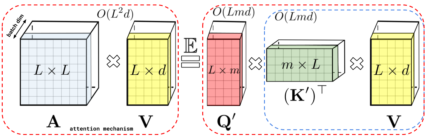 Fig.
Fig.
- Space Complexity : \(O(Lr + Ld + rd)\)
- Time Complexity : \(O(Lrd)\)
Prefix-Sum Computation
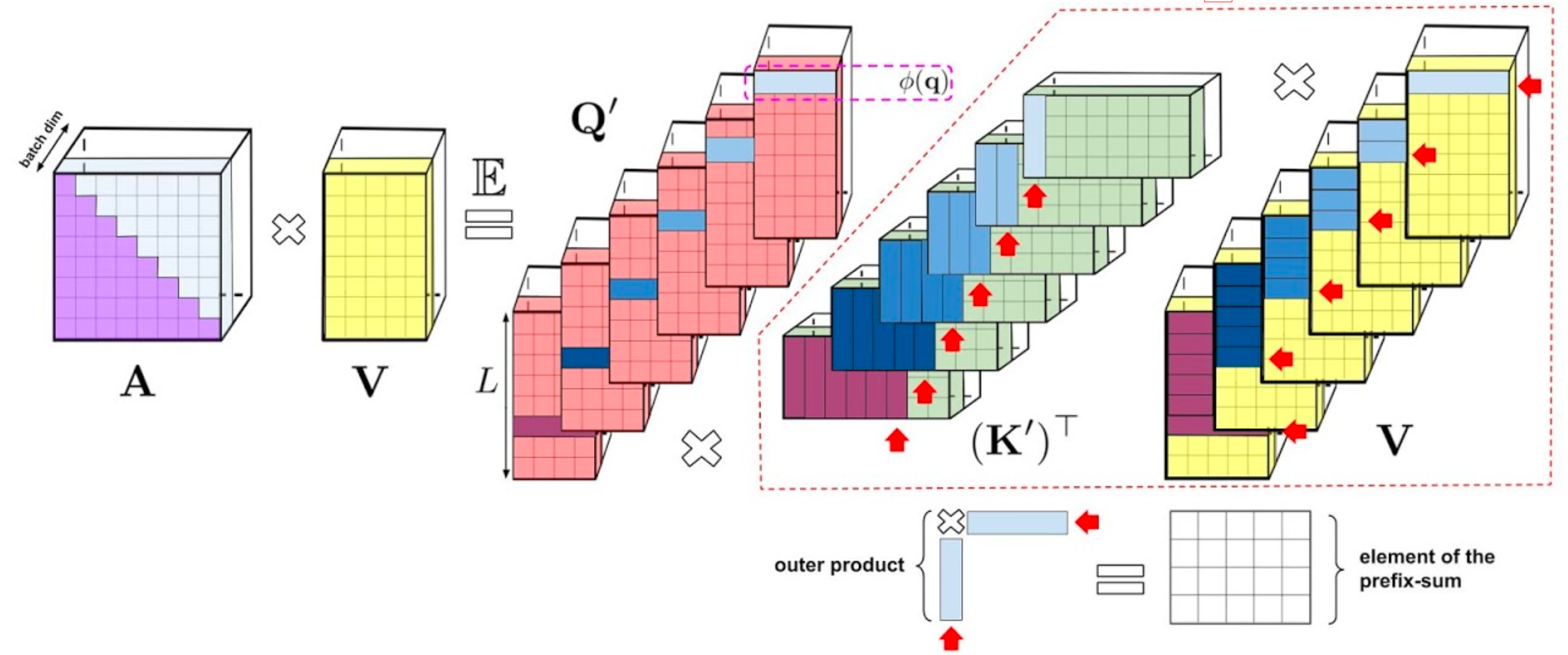 Fig.
Fig.
 Fig.
Fig.
R+ part of FAVOR+ (How to and How not to Approximate Softmax-Kernels for Attention)
 Fig.
Fig.
O part of FAVOR+ (Orthogonal Random Features (ORFS))
Theoretical Results
Pseudocode for FAVOR+
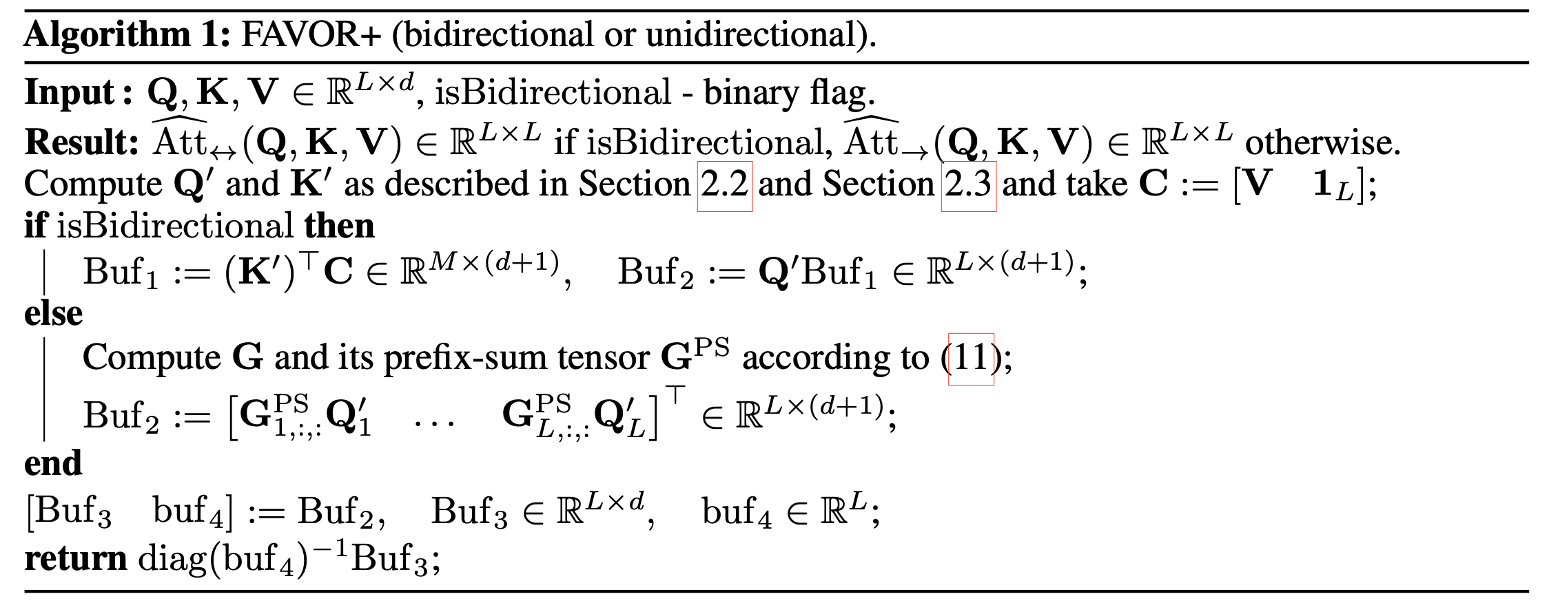 Fig.
Fig.
Experimental Results of FAVOR+
 Fig.
Fig.
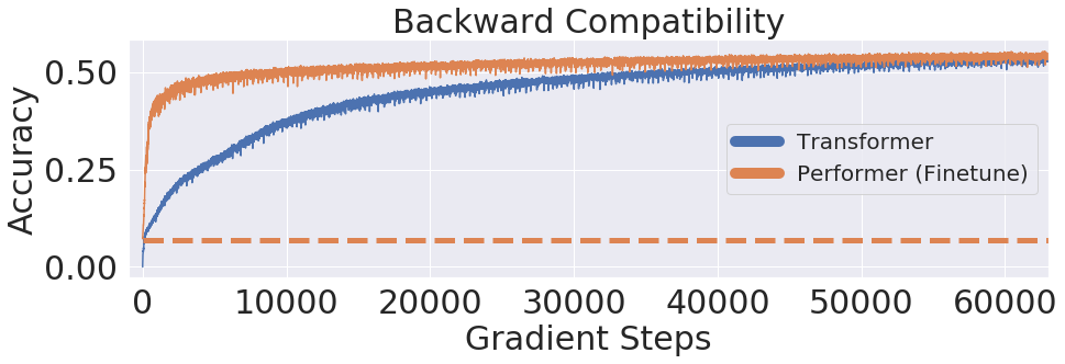 Fig.
Fig.
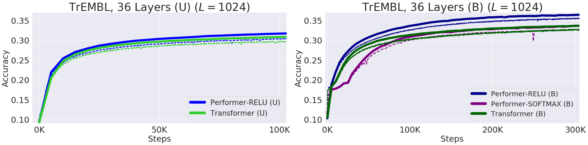 Fig.
Fig.
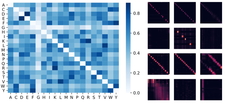 Fig.
Fig.
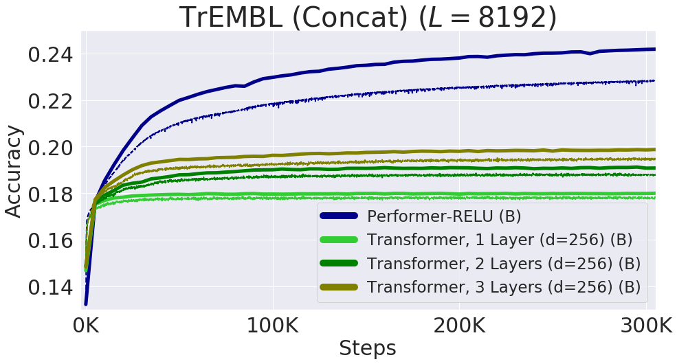 Fig.
Fig.
Long Range Arena
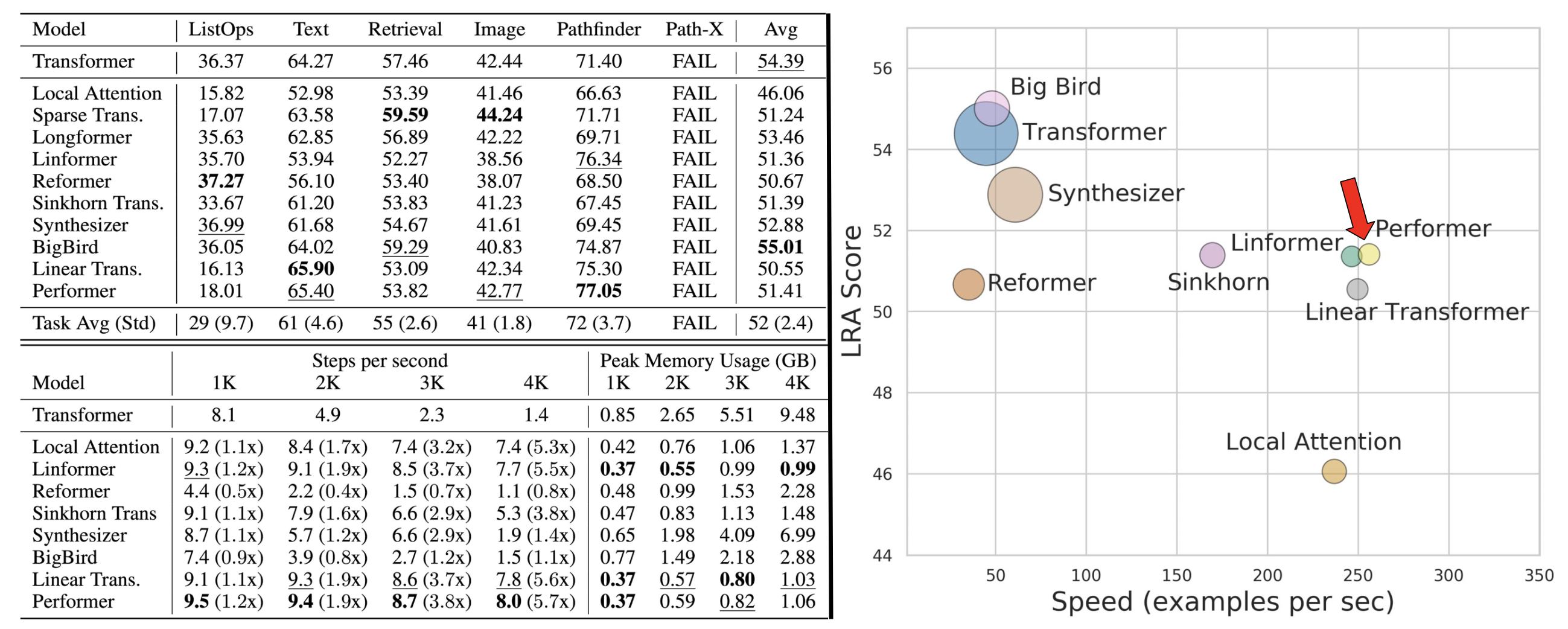 Fig.
Fig.
Connection to Linformer
Analysis on Rank of Sefl-Attention
Diagonlaization and Singular Vector Decomposition (SVD)
\[M_{m \times m}=P_{m \times m} D_{m \times m} P_{m \times m}^{-1}\] \[\begin{aligned} M & =P D P^{-1} \\ M(P) & =P D P^{-1}(P) \\ M P & =P D \end{aligned}\] \[\begin{aligned} & P=\left[a_1, a_2, \ldots a_m\right] \\ & D=\left[\begin{array}{cccc} \lambda_1 & 0 & \ldots & \ldots \\ 0 & \lambda_2 & 0 & \ldots \\ \vdots & \ldots & \ddots & \ldots \\ 0 & \ldots & 0 & \lambda_m \end{array}\right] \\ & P D=\left[\lambda_1 a_1, \lambda_2 a_2, \ldots \lambda_m a_m\right] \\ & \end{aligned}\]하지만 모든 행렬에 대해 Diagonalization 을 수행할 수 있는건 (diagonlizable) 아닌데요, 즉 행렬 \(M\) 의 크기가 정사각형 \(n \times n\) 이어야 하며 Invertible 한 경우에만 이 연산이 가능합니다. 이를 해결하기 위해 Singular Vecotr Decomposition (SVD) 를 사용할 수 있는데요,
어떤 행렬 \(M\) 에 대해서 SVD 를 수행하면 아래와 같이 \(U,S,V\) 행렬을 얻을 수 있게 됩니다.
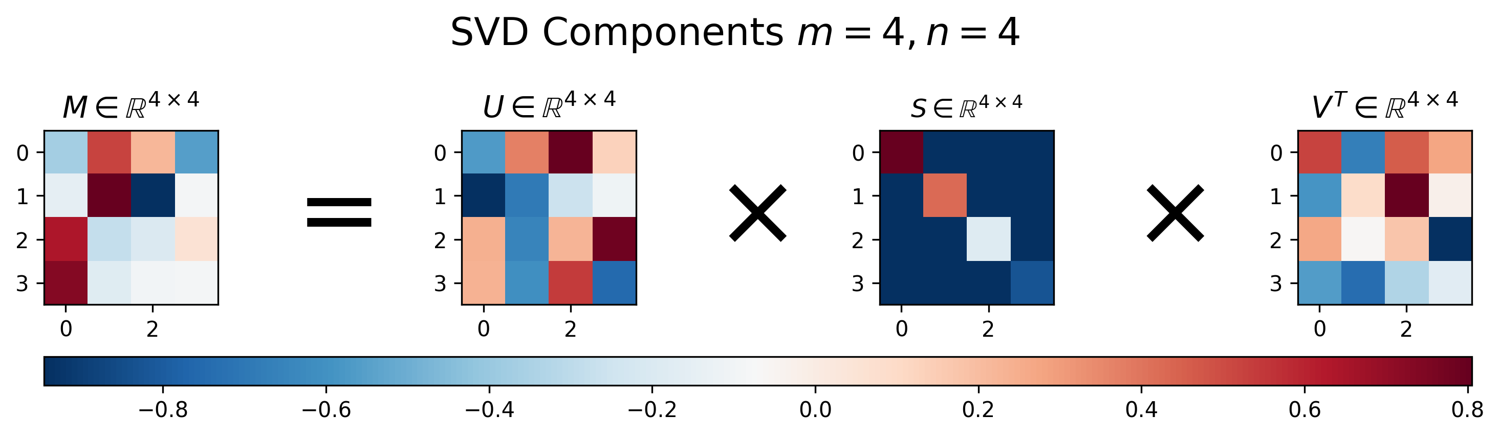
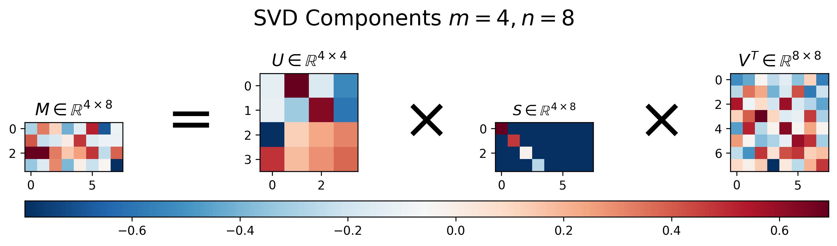
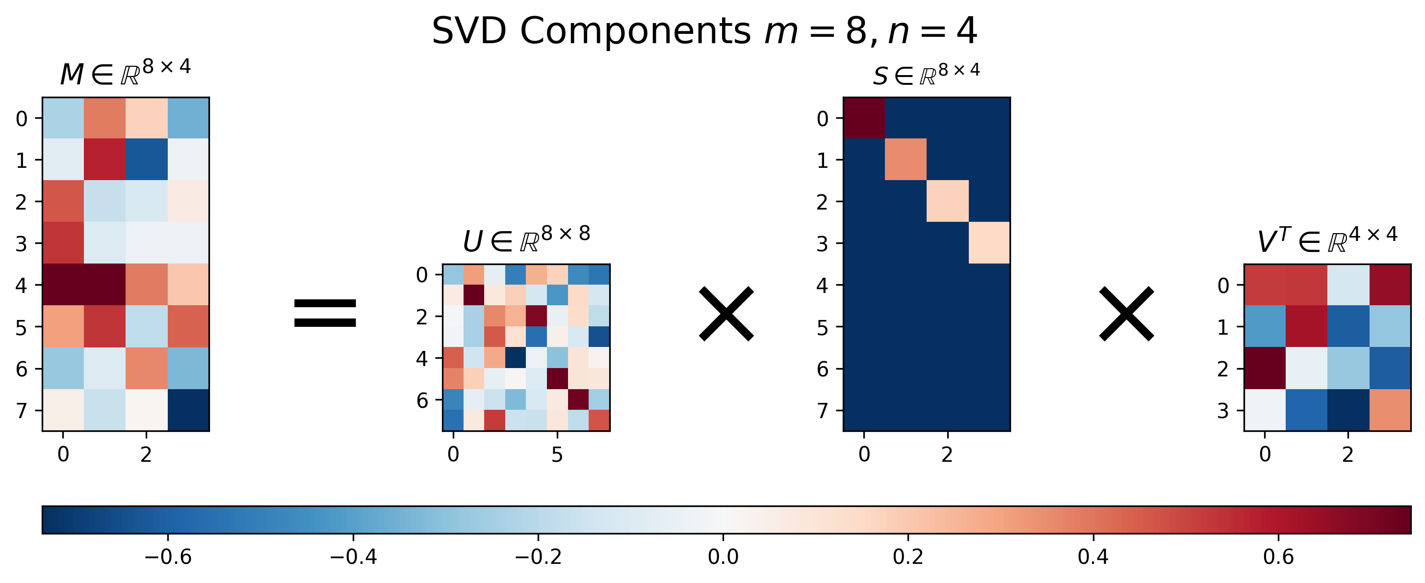 Fig. Vissualization of Results of SVD. Source From here
SVD 의 결과물을 보면 몇 가지 특이한 점을 알 수 있는데요, 바로
- U와 V의 모든 Column Vector 들은 크기 (norm) 가 1이다.
- U와 V의 Column Vector 들 간의 내적 (inner product) 을 취한 n x n Matrix 는 Identity Matrix 이다.
- U는 원본 행렬 M 의 \(MM^T\) 의 Eigenvector 를 가지고 있다.
- V는 원본 행렬 M 의 \(M^TM\) 의 Eigenvector 를 가지고 있다.
- S는 \(M^TM\) 와 \(MM^T\) 와 관련된 Eigenvalue 의 sqaure root 를 가지고 있다.
입니다.
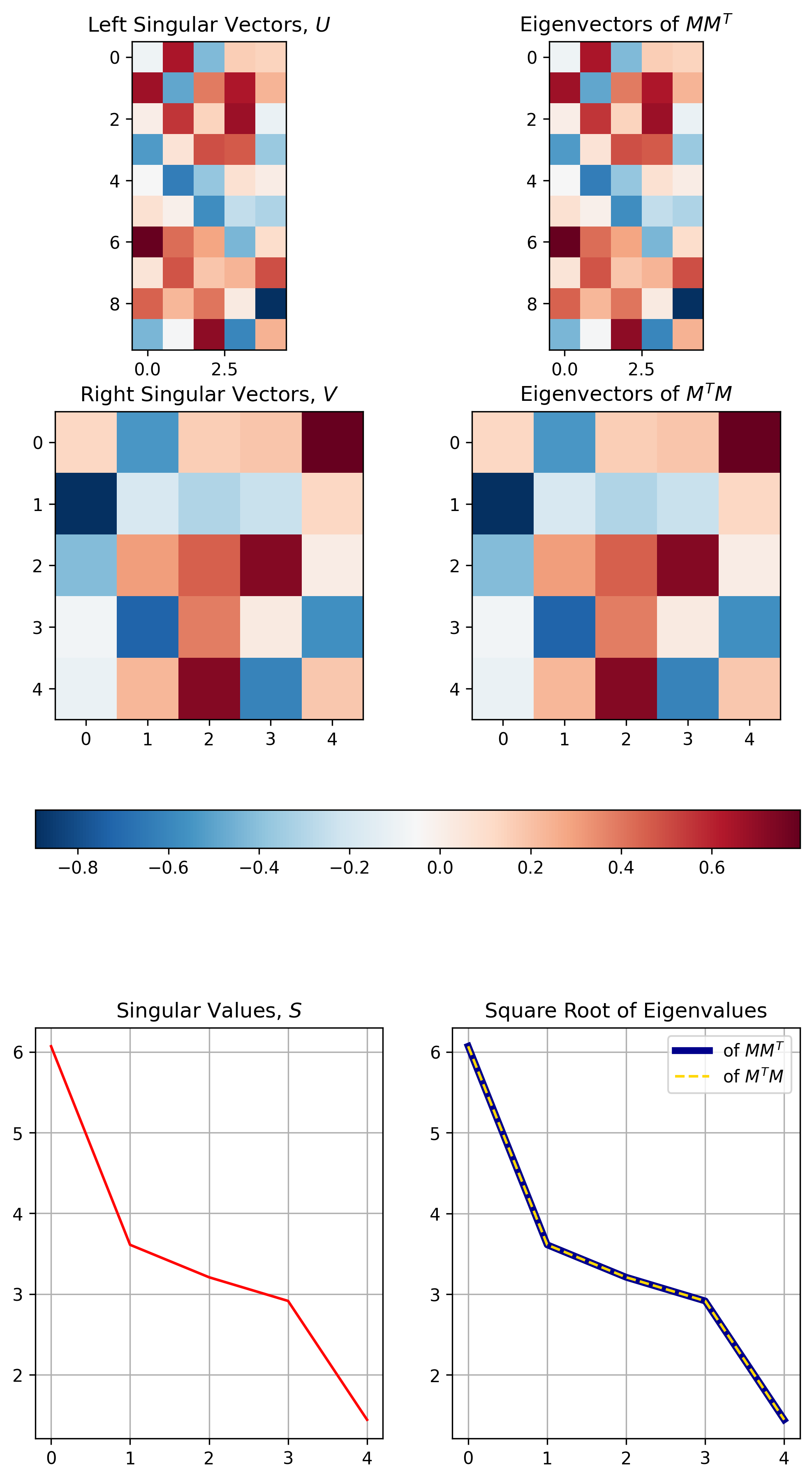 Fig. Eigenvalue Decomposition 과 SVD 의 관계. Source From here
SVD 를 잘 사용하면 여러 장점이 있지만 그 중에서 Low-Rank Matrix Approximation (LRA) 이라는 것이 가능해 집니다.
이는 \(US\) 와 \(V\) Matrix 들을 더 작은 크기의 Matrix 로 바꾸는 것인데요, SVD는 만약 Matrix 가 \(4 \times 4\) 일 경우 \(U \in \mathbb{R}^{4 \times 4}\), \(S \in \mathbb{R}^{4 \times 4}\), \(V \in \mathbb{R}^{4 \times 4}\) 를 얻을 수 있었죠,
하지만 우리는 이를 아래처럼 근사할 수 있습니다.
\[\begin{aligned} M & \approx U_k S_k V_k^T, \text{ where } k = 2 \\ & \approx \hat{M}_k \end{aligned}\]즉 우리는 \(U \in \mathbb{R}^{4 \times 2}\), \(S \in \mathbb{R}^{2 \times 2}\), \(V \in \mathbb{R}^{2 \times 4}\) 를 얻을 수 얻게 되는 건데요, 단순히 Matrix 가 Full Rank 일 때, 즉 Column 이 4일 때 Rank 가 4 인 경우에 이런 근사를 해버리면 좋지 않겠지만 우리가 만약 \(8 \times 8\) 크기의 행렬이지만 Rank 가 4 밖에 안되는 행렬을 가지고 있다면
![]() Fig. Matrix with Redundant Columns. Source From here
Fig. Matrix with Redundant Columns. Source From here
원래의 SVD를
\[\begin{aligned} M & =U S V^T \\ & =(U S) V^T \\ & =L R^T, \text { where } \\ L & =(U S), \text { and } \\ R & =V \end{aligned}\]근사해버려도 된다는 겁니다.
\[\begin{aligned} M & =L R^T \\ & \approx L_k R_k^T \\ & \approx \hat{M} \end{aligned}\]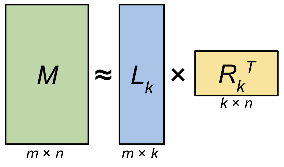 Fig. \(m \times n\) 크기의 Matrix \(M\) 을 \(m \times k\), \(k \times n\) 로 분해할 수 있다. 만약 \(k\) 가 데이터의 rank \(r\) 과 같다면 (\(r=k\)) Matrix \(M\) 은 완전히 Decomposition 으로부터 복원될 수 있고 \(k\)가 \(r\)보다 작으면, 즉 \(k<r\) 이면 근사된 Matrix, 즉 Low-Rank Approximated Matrix \(\hat{M}\) 을 얻을 수 있다.. Source From here
이렇게 근사를 해서 얻은 \(L, R (U,S,V)\) 를 사용해도 Redundant Column 이 포함되어 있는 행렬 \(\tilde{X}\) 를 복구하는데는 문제가 없다고 합니다.
![]() Fig. . Source From here
Fig. . Source From here
Self-Attention is Low Rank
한편 우리가 Transformer 에서 근사하고 싶은 연산은 \(QK^T\) 연산 이었습니다.
\[P = \text{softmax} [ \frac{QW_i^Q (KW_i^K)^T}{\sqrt{d}} ] = \exp (A) \cdot D_A^{-1}\]Performer 논문에서와 같이 \(D_A\) 는 \(n \times n\) 의 diagonal matrix 이며, Self Attention 을 위와 같이 나타낼 때 \(QK^T\) 행렬은 Sequence Length \(L\)에 대해 \(L^2\) 만큼의 연산량이 드는 것으로 \(A \in \mathbb{R}^{L \times L}\) 크기를 갖는데요, Linformer 에서는 이를 Eigenvalue 를 사용해 분석해봤습니다.
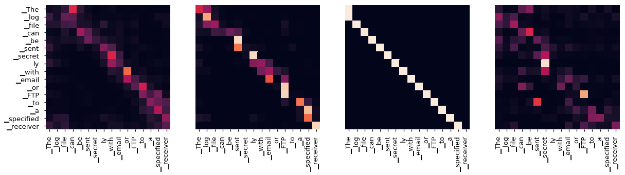 Fig. Visualization of Self Attention of Transformer Encdoer 2nd Layer. Source from here
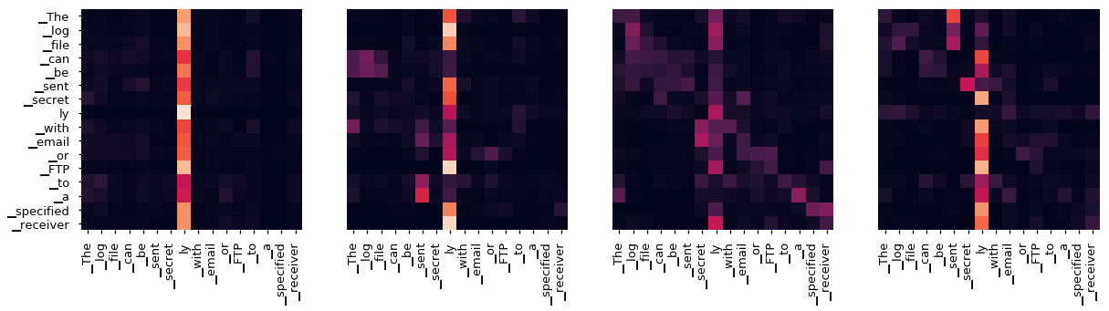 Fig. Visualization of Self Attention of Transformer Encdoer 6th Layer. Source from here
(논문에서는 Masked Language Modeling (MLM) 방식으로 학습된 Transformer Encoder Only Model, RoBerta 를 분석했지만 제가 가지고 온 Figure 는 Encoder-Decoder 구조의 번역 데이터를 학습 한것이라는 점을 인지해 주시기 바랍니다.)
논문에서는 Transformer 의 층별로 존재하는 12개 Head 들에서 계산된 Context Mapping Matrix (\(QK^T\) 계산을 하고 Scailing 한 것을 Row-wise 로 Normalization 한 것), P를 SVD 연산을 합니다.
이를 10,000개 Setences 에 대해서 한 뒤 누적시켜서 평균을 내고 Normalization 를 한 Normalized Cumulative Singular Value Averaged over 10k Sentences 값을 구해서 결과를 봤는데요
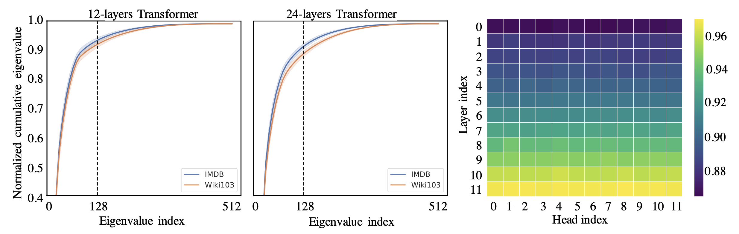 Fig. Spectrum Analysis of the Context Mapping Matrix. 오른쪽은 전체 512개 Token 중에서 128번째로 큰 Singular Value 에서의 Normalized Cumulative Singular Value 에 대한 Heatmap
그 결과 얻은 각 Layer, Head 별로 Long-tail Spectrum Distribution 을 얻었다고 합니다.
이는 대부분의 Attention Map, \(P\) 는 처음 몇개의 큰 Singular Value 들만 있으면 복원이 된다는 것이죠.
이러한 현상은 낮은 Layer 보다 높은 Layer 에서 두드려졌다고 하는데요, 즉 위로 갈수록 Information 이 한쪽으로 집중되는 현상이 컸다는 겁니다. \(P\) 의 Rank 가 갈수록 낮았던 거죠.
Linformer Method
이러한 Encoder 의 Self Attention 은 Low Rank 라는 특성을 이용해 저자들은 Layer 와 Head 별로 \(E_i, F_i \in \mathbb{R}^{n \times k}\) 라는 두 개의 Linear Projection Matrix 를 도입해서 K, V 를 계산할 때 쓰기로 하는데요,
즉 사실상 Performer 과 거의 유사하게 Attention Score Map 을 Approximation 을 해버립니다.
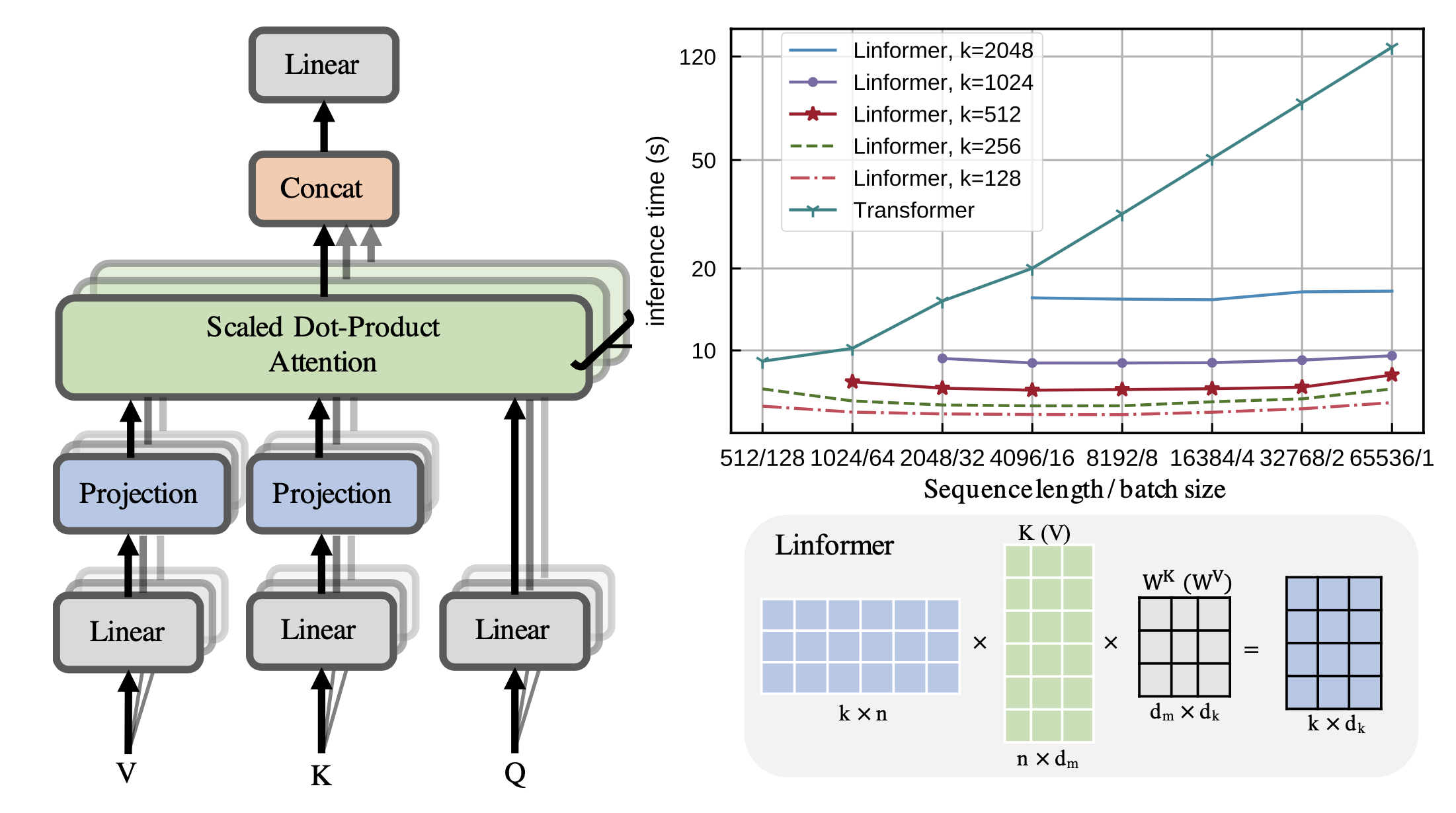 Fig.
Fig.
Performer vs Linformer
Performer 와 Linformer 의 차이는 첫 번째로
 Fig.
Fig.
 Fig.
Fig.
 Fig.
Fig.
Pytorch Implementation
Performer
Source from lucidrains’ implementation
# non-causal linear attention
def linear_attention(q, k, v):
    k_cumsum = k.sum(dim = -2)
    D_inv = 1. / torch.einsum('...nd,...d->...n', q, k_cumsum.type_as(q))
    context = torch.einsum('...nd,...ne->...de', k, v)
    out = torch.einsum('...de,...nd,...n->...ne', context, q, D_inv)
    return out
# efficient causal linear attention, created by EPFL
# TODO: rewrite EPFL's CUDA kernel to do mixed precision and remove half to float conversion and back
def causal_linear_attention(q, k, v, eps = 1e-6):
    from fast_transformers.causal_product import CausalDotProduct
    autocast_enabled = torch.is_autocast_enabled()
    is_half = isinstance(q, torch.cuda.HalfTensor)
    assert not is_half or APEX_AVAILABLE, 'half tensors can only be used if nvidia apex is available'
    cuda_context = null_context if not autocast_enabled else partial(autocast, enabled = False)

    causal_dot_product_fn = amp.float_function(CausalDotProduct.apply) if is_half else CausalDotProduct.apply

    k_cumsum = k.cumsum(dim=-2) + eps
    D_inv = 1. / torch.einsum('...nd,...nd->...n', q, k_cumsum.type_as(q))

    with cuda_context():
        if autocast_enabled:
            q, k, v = map(lambda t: t.float(), (q, k, v))

        out = causal_dot_product_fn(q, k, v)

    out = torch.einsum('...nd,...n->...nd', out, D_inv)
    return out
class FastAttention(nn.Module):
    def __init__(self, dim_heads, nb_features = None, ortho_scaling = 0, causal = False, generalized_attention = False, kernel_fn = nn.ReLU(), no_projection = False):
        super().__init__()
        nb_features = default(nb_features, int(dim_heads * math.log(dim_heads)))

        self.dim_heads = dim_heads
        self.nb_features = nb_features
        self.ortho_scaling = ortho_scaling

        self.create_projection = partial(gaussian_orthogonal_random_matrix, nb_rows = self.nb_features, nb_columns = dim_heads, scaling = ortho_scaling)
        projection_matrix = self.create_projection()
        self.register_buffer('projection_matrix', projection_matrix)

        self.generalized_attention = generalized_attention
        self.kernel_fn = kernel_fn

        # if this is turned on, no projection will be used
        # queries and keys will be softmax-ed as in the original efficient attention paper
        self.no_projection = no_projection

        self.causal = causal
        if causal:
            try:
                import fast_transformers.causal_product.causal_product_cuda
                self.causal_linear_fn = partial(causal_linear_attention)
            except ImportError:
                print('unable to import cuda code for auto-regressive Performer. will default to the memory inefficient non-cuda version')
                self.causal_linear_fn = causal_linear_attention_noncuda

    @torch.no_grad()
    def redraw_projection_matrix(self, device):
        projections = self.create_projection(device = device)
        self.projection_matrix.copy_(projections)
        del projections

    def forward(self, q, k, v):
        device = q.device

        if self.no_projection:
            q = q.softmax(dim = -1)
            k = torch.exp(k) if self.causal else k.softmax(dim = -2)

        elif self.generalized_attention:
            create_kernel = partial(generalized_kernel, kernel_fn = self.kernel_fn, projection_matrix = self.projection_matrix, device = device)
            q, k = map(create_kernel, (q, k))

        else:
            create_kernel = partial(softmax_kernel, projection_matrix = self.projection_matrix, device = device)
            q = create_kernel(q, is_query = True)
            k = create_kernel(k, is_query = False)

        attn_fn = linear_attention if not self.causal else self.causal_linear_fn
        out = attn_fn(q, k, v)
        return out
References
- Papers
- Rethinking Attention with Performers
- Reformer: The Efficient Transformer
- Transformer with Fourier Integral Attentions
- Skyformer: Remodel Self-Attention with Gaussian Kernel and Nyström Method
- Long Range Arena: A Benchmark for Efficient Transformers
- Linformer: Self-Attention with Linear Complexity
- Relative Positional Encoding for Transformers with Linear Complexity
- Blogs
- Others
- Computational Complexity of Self-Attention in the Transformer Model (Stackoverflow)
- SVD and Data Compression Using Low-rank Matrix Approximation from Dustin Stansbury
- Singular Value Decomposition: The Swiss Army Knife of Linear Algebra from Dustin Stansbury
- What is an intuitive explanation of the rank of a matrix? (Qoura)
- Implementation