Generative Adversarial Networks (GANs)
03 Dec 2022< 목차 >
- What's difference between Variational Auto Encoder (VAE) and Generative Adversrial Network (GAN)
- GAN
- Improved GAN Training
- References
What's difference between Variational Auto Encoder (VAE) and Generative Adversrial Network (GAN)
Generative Adversarial Networks (GANs) 이 어떻게 학습되는지? 에 대해 이야기 하기 전에, 우리는 ‘생성 모델이란 무엇인가?’, ‘생성 모델에는 어떤 종류가 있는가?’, ‘GAN 은 어떻게 탄생했으면 어떤 장점 때문에 다른 생성 모델을 대체하는가?’ 에 대해서 생각해 보도록 합시다.
Recap VAE (Latent Variable Model, Explicit Model)
우리가 앞서 배운 Varitaional Auto Encoder (VAE) 같은 생성 모델 (Generative model)의 목적은 뭘까요?
바로 실제 data point (sample) 들이 어떤 분포에서 sampling 됐을까? 그 분포를 추정해보자 입니다.
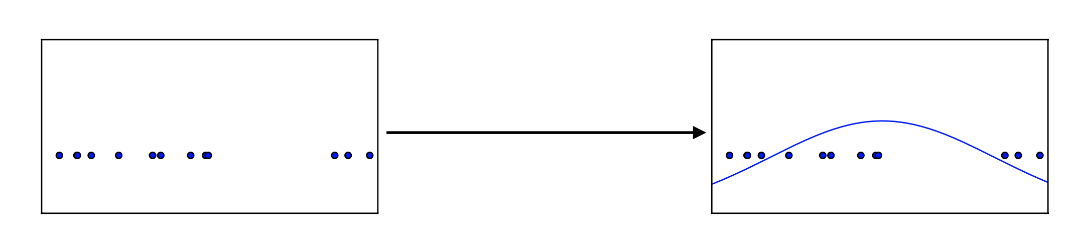 Fig. Maximum Likelihood Estimation
이 때 데이터의 실제 분포는 \(p_{data}\) 라고 하는데요, 당연히 우리는 이 분포가 어떻게 생겼는지 모릅니다.
그렇기에 대부분의 경우 우리는 \(p_{data}\) 라는 확률 분포, 즉 Likelihood를 최대화 하기 위해서 보통 이 분포가 어떻게 생겼는지를 가정하고 이에 맞는 Objective 를 만들게 됩니다.
이 때 이 Target Distribution이 Gaussian Distribution 이라면 MSE Loss가, Bernoulli 나 Categoriacal Distribution 이라면 (Binary) Cross Entropy Loss 가 도출되게 됩니다.
VAE는 이 Likleihood 의 모양이 어떻든 데이터 내에 잠재 변수 \(z\) (or \(h\)라고 쓰는 논문도 많음) 를 정하고 이 Likelihood 를 최대화 하려고 하며 이 때 바로 변분 추론 (Variatioanl Approximation) 이 들어가게 되고 결국 Evidence Lower Boundary (ELBO) term 을 Objective로 얻게 됩니다.
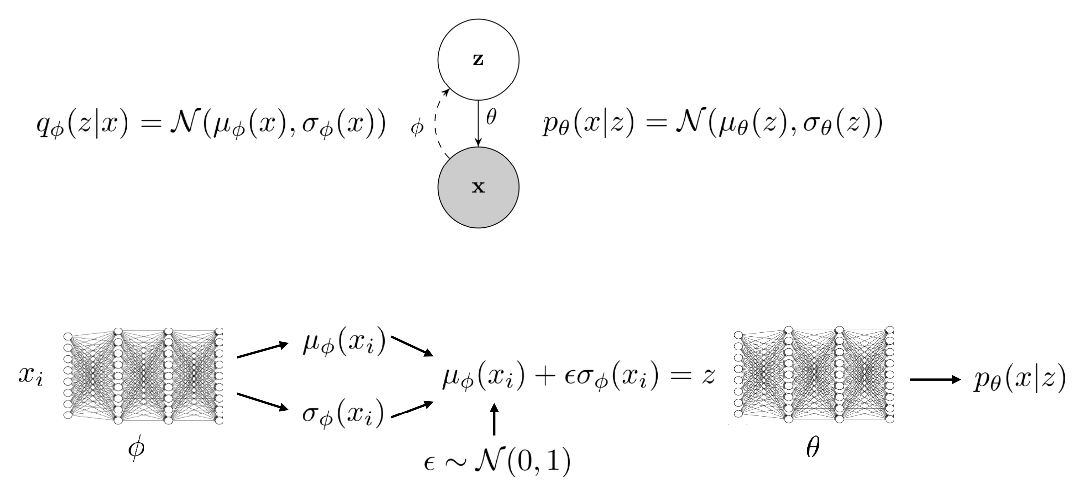 Fig. Graphical Model of Variational Auto Ecndoer (VAE)
여기서 Objective 는 사실상 MSE + Regularization 라는것을 알 수 있는데요, 이는 이미지가 대부분 continuous value 이기 때문에 대부분 Gaussian 을 Target 으로 삼아서 그렇습니다. (흑 백 이미지의 경우 Bernoulli 를 Target으로 해서 Binary Classification Task 로도 학습할 수 있습니다.)
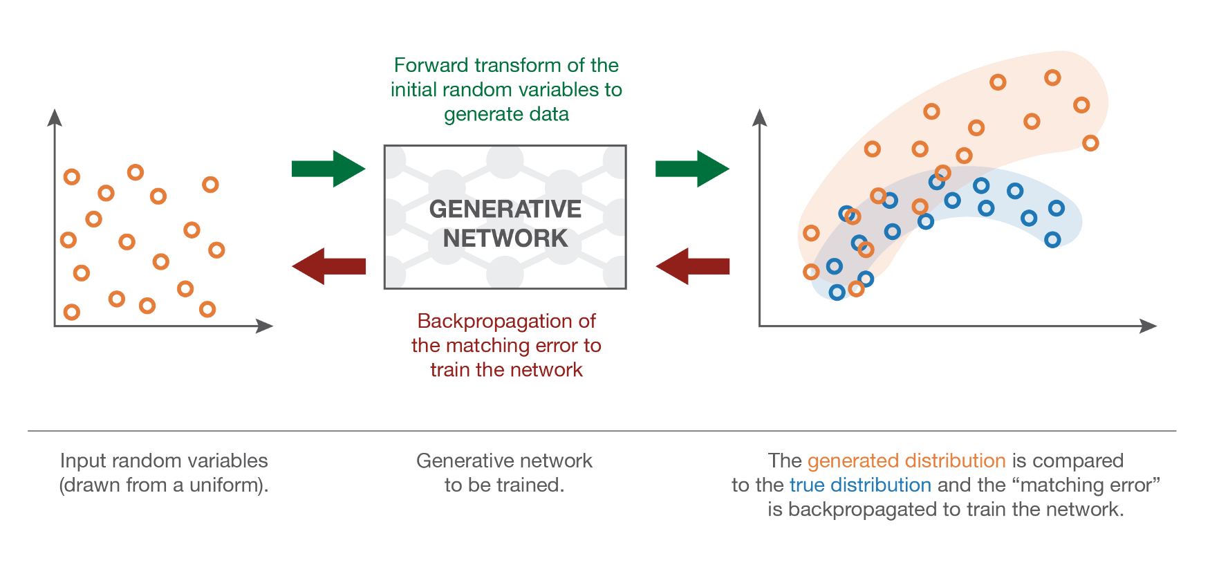 Fig. VAE 를 학습하는 것은 결국 실제 데이터 분포가 어떤지를 가우시안일 것이라고 생각하고 가우시안의 파라메터를 fitting 함으로써 실제 분포와 매칭시키는 것으로 생각할 수 있다.
위의 Objective 에서도 알 수 있지만 VAE 를 학습해서 실제 Inference 할 때에는 random vector \(z\) 를 받아 이미지로 변환해 줄 Decoder \(p_{\theta}\) 만 있으면 되는데요,
실제 학습할 때에는 이 디코더를 학습하기 위해 \(q_{\phi}\) 라는 Encoder가 부수적으로 필요합니다.
왜냐하면 VAE는 실제 이미지를 Latent Space 에 매핑하고 그렇게 의미있게 매핑된 Space 에서 샘플링한 noise vector를 디코더가 사용해 학습하기 때문이죠.
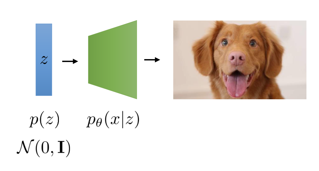 Fig. Inference 시에는 Decoder만 있으면 되는 VAE
Explicit Density Models vs Implicit Density Model
우리가 앞으로 알아보게 될 GAN 도 random vector \(z\) 를 샘플링하고 Decoder 가 이를 이미지화 하는 것은 같습니다.
그리고 내가 가지고 있는 데이터들이 어떤 분포에서 샘플링 됐을까? 이걸 찾고싶다 라는 Goal 또한 같습니다.
하지만 VAE와 GAN이 가지는 큰 차이점들이 몇가지 있고 이에 따라 모델이 만들어내는 새로운 샘플 (새로운 이미지, 음성) 등의 퀄리티도 다른데요, 그 중 두가지는
- GAN은
Target Distribution을 설정하지 않지만 결국 데이터 분포를 찾아낸다 - Encoder 가 존재하지 않고 대신
다른 모듈이 있다.
라는 겁니다.
여기서 다른 모듈은 바로 Discriminator, \(D\) 라는 네트워크로 GAN 의 적대적인 두 신경망 중 하나입니다.
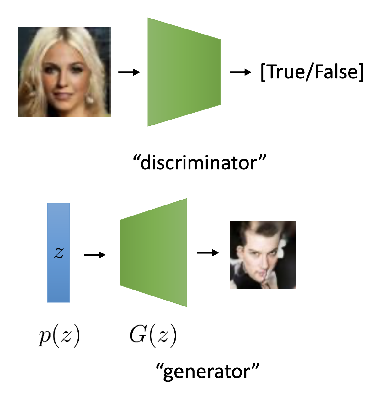 Fig.
Fig.
곧 살펴보겠지만, GAN의 Training Objective 는 아래와 같은데요,
\[\min _G \max _D V(D, G)=E_{x \sim p_{\text {data }}(x)}[\log D(x)]+E_{z \sim p(z)}[\log (1-D(G(z)))]\]여기서 G 가 바로 Generator, 즉 noise vector를 받아 이미지화 하는 Decoder 입니다.
VAE 에서는 \(p(x \vert z)\), 즉 \(G(z)\) 를 가우시안 분포로 정하고 이 Likelihood를 최대화 했었습니다.
하지만 GAN은 어떨까요? 일단 우리가 실제로 추론 시 필요한 것은 G 이니까 이것이 포함되어있는 우변의 2번째 항만 보면
디코딩된 이미지를 다시 Discriminator, D 에 들어가고 이 D의 출력값 (확률) 이 커지게 학습이됩니다.
여기서 Generator가 만든 이미지를 D가 받고 이것의 출력값이 커지게 (1에 가깝게) 학습된다는 것은 무슨 의미일까요? 바로 모델이 만들어낸 이미지를 진짜에 가깝게 판독하게끔 D와 G의 파라메터를 동시에 업데이트 하라는 뜻이 됩니다.
실제로 학습이 잘 되면 D는 어떤 이미지가 들어와도 진짜인지 가짜인지 구분할 수 없어야 하는데요, 즉 네트워크가 만든 것도 \((0.5, 0.5)\) 확률을, 실사 이미지를 넣어도 \((0.5, 0.5)\) 의 Binary 확률을 뱉어야 합니다.
중요한 점은 이 때 우리가 \(G(z)\) 가 어떤 분포인지 정하지 않았다는 겁니다.
즉 \(- log G(z)\) 라는 Negative Log Likelihood 를 직접적으로 최대화 하지 않고, \(\log (1-D(G(z)))\) 를 사용해서 G 를 학습하는 겁니다.
이 부분이 바로 결정적인 차이점 인데요,
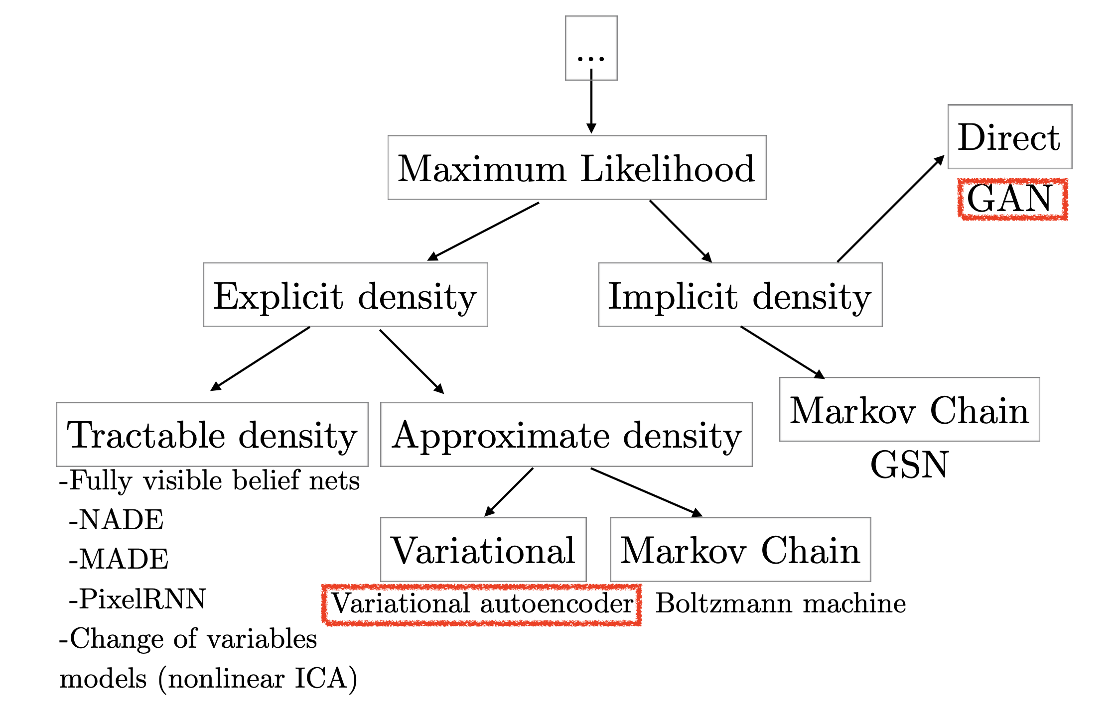 Fig. Generative Model Taxonomy
라고 정하고 이를 최대화 하려고 했던 VAE 는 명시적 (explcit) 하게 모델의 Target Density 을 정한 것 이므로 Explicit Density Model 라고 부르고
GAN 은 Target Density를 따로 정하지 않았지만 데이터의 분포를 알아서 배우는, 이른 바 Implicit Density Model이라고 불립니다.
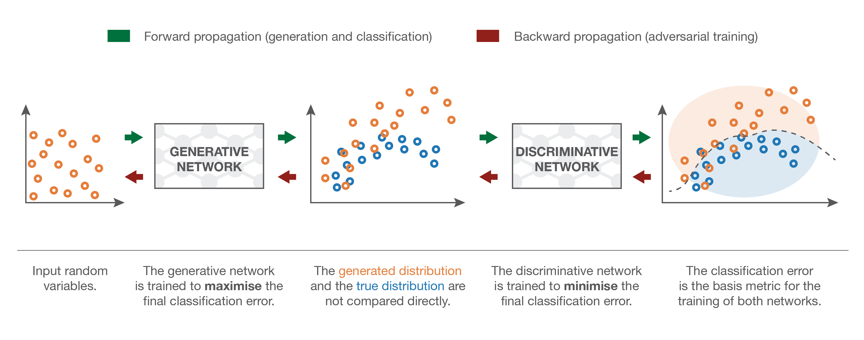 Fig. What GANs Learn ?
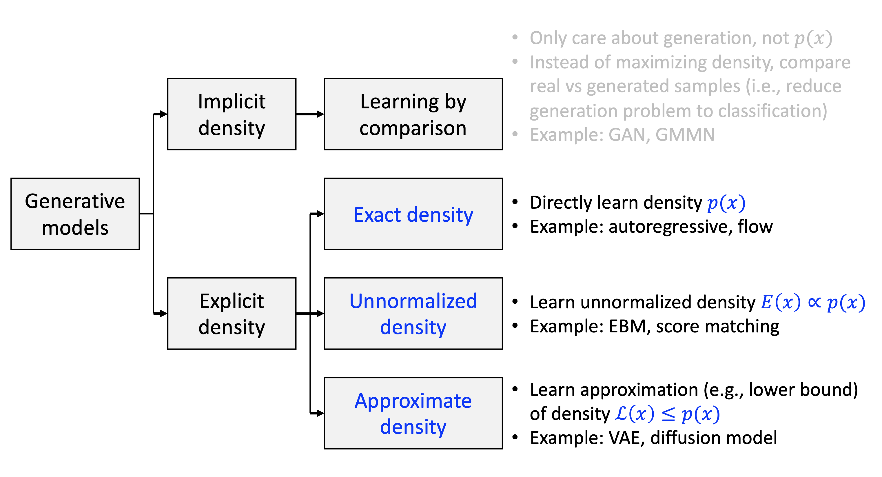 Fig. Explicit vs Implicit Density Model. Source From KAIST AI602 Lecture 5 Slide
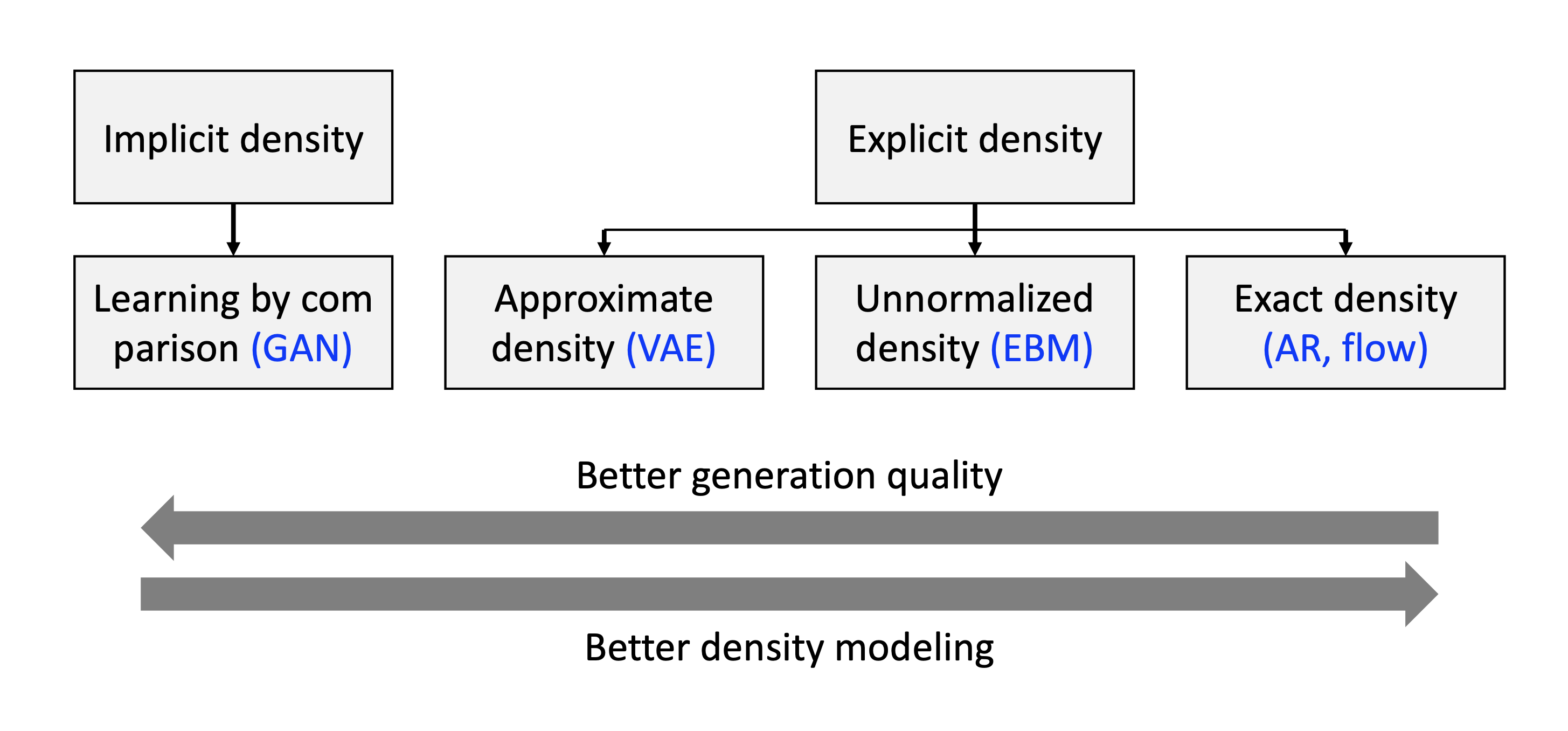 Fig. Explicit vs Implicit Density Model 2. Source From KAIST AI602 Lecture 5 Slide
GAN
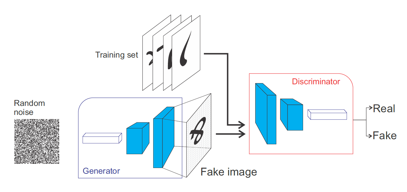 Fig. Vanilla GAN.
2 가지 중요한 사항이 있는데요 바로,
- 1.How to make this work with stochastic gradient descent/ascent?
- 2.How to compute the gradients?
입니다.
What does the GAN optimize ?
GAN architectures
Improved GAN Training
Why is training GANs hard? and How can we make it better?
Mode Collapse
Wasserstein GAN (WGAN)
- Least-squares GAN (LSGAN) : discriminator outputs real-valued number
Wasserstein GAN (WGAN): discriminator is constrained to be Lipschitz-continuous- Gradient penalty : discriminator is constrained to be continuous even harder
Spectral norm: discriminator is really constrained to be continuousInstance noise: add noise to the data and generated samples
References
- Generative Adversarial Networks
- NIPS 2016 Tutorial: Generative Adversarial Networks
- CVPR 2018 Tutorial on GANs
- Google Doc. Machine Learning > Advanced courses > GAN
- Generative adversarial networks from julien-vitay
-
Understanding Generative Adversarial Networks (GANs) from Joseph Rocca
- Lecture Videos