(almost) Pytorch Efficient Scaled Dot Product Attention (SDPA)

< 목차 >

Motivation
Technical Explanation of Efficient Scaled Dot Product Attention (SDPA)
- Memory Efficient SDPA (xformers)
- Flash Attention
Implementation of Efficient SDPA
How to Inject Relative Positional Information in xformers
- Attention Bias (ALiBi or TFXL RPE)
- RoPE
Benchmarks on Real-World Model and Dataset
- RoBERTa Large
References

Motivation

대부분의 논문 구현체들이 최적화 된 상태로 제공되지는 않는다. 그것이 Big Tech 에서 공개한 것이더라도 말이다. 예시로 유명한 Open-source 구현체들을 몇 개 봐보도록 하자. 아래는 Facebook AI Research (FAIR) 의 Sequence-to-sequence task 들을 위한 open-source library, fairseq의 multihead attention 구현체의 코드 중 일부이다.

class MultiHeadAttention(nn.Module):
    def __init__(self, n_feat, n_head, dropout):
        """Construct an MultiHeadedAttention object."""
        super(ESPNETMultiHeadedAttention, self).__init__()
        assert n_feat % n_head == 0
        # We assume d_v always equals d_k
        self.d_k = n_feat // n_head
        self.h = n_head
        self.linear_q = nn.Linear(n_feat, n_feat)
        self.linear_k = nn.Linear(n_feat, n_feat)
        self.linear_v = nn.Linear(n_feat, n_feat)
        self.linear_out = nn.Linear(n_feat, n_feat)
        self.attn = None
        self.dropout = nn.Dropout(p=dropout)

    def forward_qkv(self, query, key, value, **kwargs):
        n_batch = query.size(0)
        q = self.linear_q(query).view(n_batch, -1, self.h, self.d_k)
        k = self.linear_k(key).view(n_batch, -1, self.h, self.d_k)
        v = self.linear_v(value).view(n_batch, -1, self.h, self.d_k)
        q = q.transpose(1, 2)  # (batch, head, time1, d_k)
        k = k.transpose(1, 2)  # (batch, head, time2, d_k)
        v = v.transpose(1, 2)  # (batch, head, time2, d_k)
        return q, k, v

    def forward_attention(self, value, scores, mask):
        n_batch = value.size(0)
        if mask is not None:
            scores = scores.masked_fill(
                mask.unsqueeze(1).unsqueeze(2).to(bool),
                float("-inf"),  # (batch, head, time1, time2)
            )
            self.attn = torch.softmax(scores, dim=-1)  # (batch, head, time1, time2)

        else:
            self.attn = torch.softmax(scores, dim=-1)  # (batch, head, time1, time2)
        p_attn = self.dropout(self.attn)
        x = torch.matmul(p_attn, value)  # (batch, head, time1, d_k)
        x = (
            x.transpose(1, 2).contiguous().view(n_batch, -1, self.h * self.d_k)
        )  # (batch, time1, d_model)

        return self.linear_out(x)  # (batch, time1, d_model)

    def forward(self, query, key, value, key_padding_mask=None, **kwargs):
        query = query.transpose(0, 1)
        key = key.transpose(0, 1)
        value = value.transpose(0, 1)

        q, k, v = self.forward_qkv(query, key, value)
        scores = torch.matmul(q, k.transpose(-2, -1)) / math.sqrt(self.d_k)
        scores = self.forward_attention(v, scores, key_padding_mask)
        scores = scores.transpose(0, 1)
        return scores, None

위 class는 Transformer 의 Multi-Head Attention (MHA)를 하는 module이다. Input sequence x에 대해서 query, key, value space로 projection하는 연산을 한 뒤에 얻은 q,k,v 를 사용해 q @ k 계산을 하고, 얻은 attention score map 을 softmax 로 normalize 해준 뒤 scaling 을 해준다. 그리고 각 value vector들과 내적을 해 주는 데(softmax(q@k / \sqrt{d_k}) @ v), q,k,v projection 이후의 모든 연산을 통 틀어서 key, value간의 similarity (dot product)를 measure 하고 scaling한다고 하기에 Scaled Dot Product Attention (SDPA)라 부른다. 그리고 마지막으로 output projection layer를 통과시키면 MHA operation을 다 한것이다.

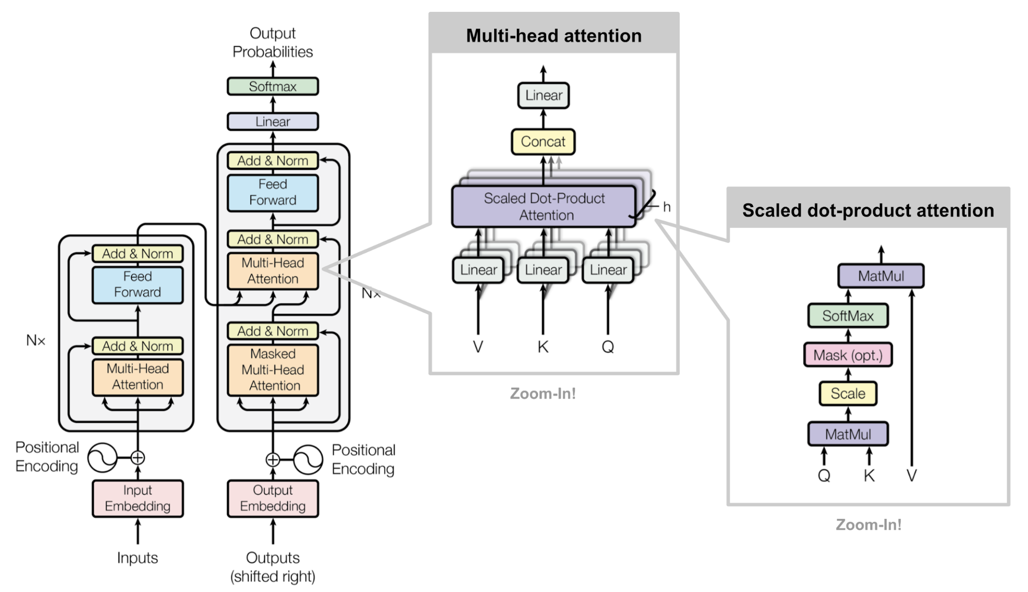sdpa Fig. Source from link

언뜻보기엔 문제없는 코드같지만 위의 코드에 문제점이 있는데, 바로 SDPA 구현이 단순해서 Time, Space complexity가 너무 크다는 것이다.

attn_weight = torch.softmax(q @ k.transpose(-2, -1) / math.sqrt(q.size(-1)), dim=-1)
out = (attn_weight @ v)

이게 무슨 소리일까?

SDPA operation은 sequence length, \(L\)의 제곱에 비례하는 (quadratic) space and time complexity를 갖는다고 알려져 있다. 하지만 이는 이론적으로 그렇다는 것이며 최신 library 들에서 제공하는 optimized SDPA를 사용하면 complexity를 확 줄일수 있다는 것이 널리 알려져 있다. 가장 큰 이유는 아래 2가지인데,

q@k 를 계산해서 memory로 저장하고 있는 행위 자체가 sequence length L에 대해 \(L^2d\) 만큼의 cuda memory를 잡아먹는다.
matmul을 한 결과를 저장하고 softmax 할 때 또 다른 memory에 올리고 또 저장했다가 value와 곱할 때 … 이런 불필요한 과정에서 I/O 시간이 추가로 발생한다.

이를 해결하기 위해서 optimized kernel을 써야 한다. 예를 들어 pytorch의 경우 version이 올라가면서 torch.nn.functional.scaled_dot_product_attention 같은 function을 포함하게 되었는데, 이 function은 내부적으로 memory efficient operation trick이나, flash attention 같은 것들이 포함되어 있어, memory도 덜 잡아먹고 속도도 훨씬 빠르다. 아마 대부분의 Open-source들은 연구용이고 서비스를 고려해서 제공할 이유까지는 없기 때문에 신경을 쓰지 않은 부분이 있는 것 같다. Open-source Large Language Model (LLM) 중 가장 유명한 LLaMa도 논문에서는 xformers를 사용해서 학습 효율을 높혔다고 하는데

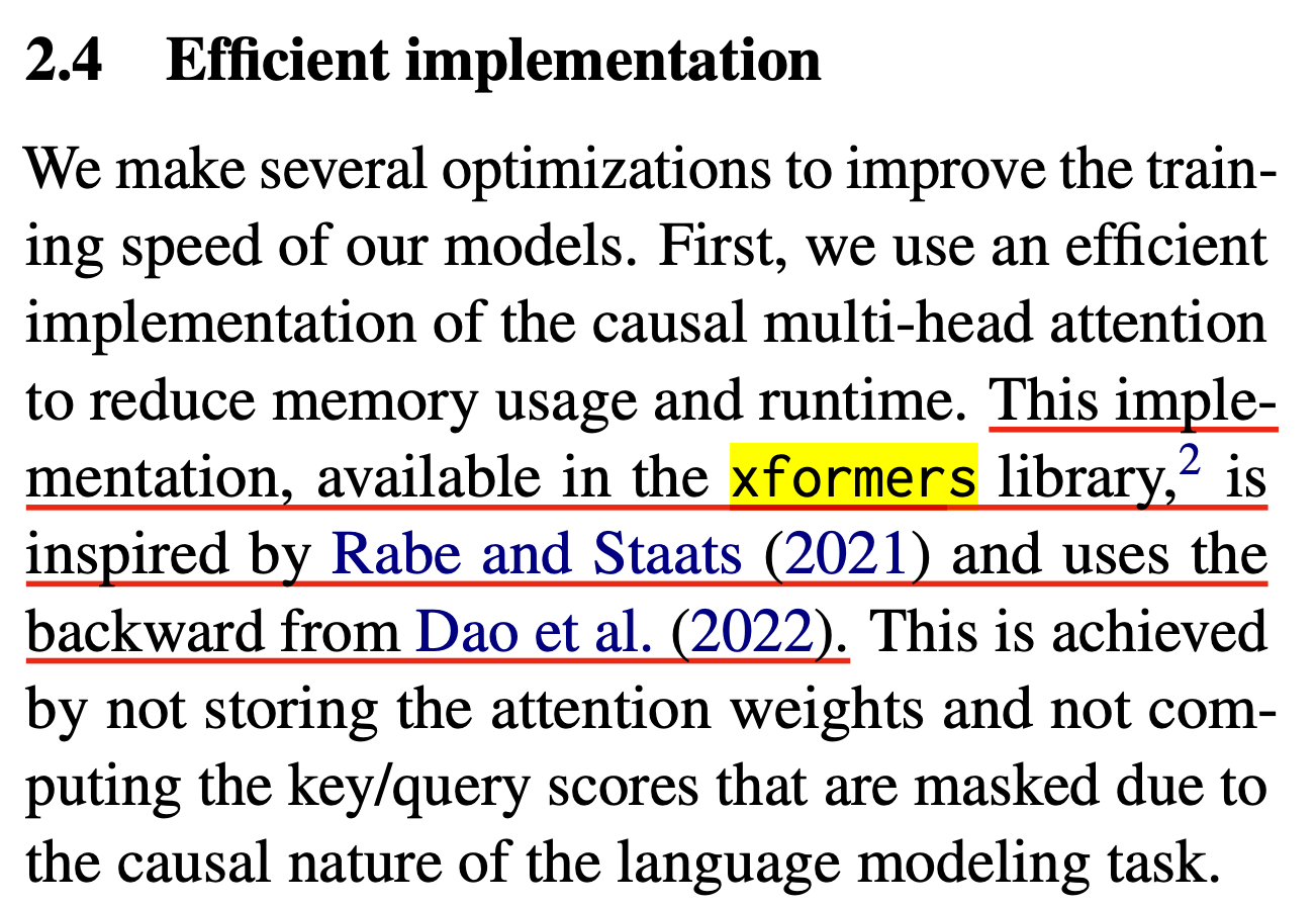llama1_xformers Fig. LLaMa 1 paper에서는 어떤식으로 학습 효율을 극대화 했는지 기술하였으나, 공개된 코드에는 이런 부분이 없다.

공개된 코드는 naive한 SDPA를 쓰고 있으니 실제 학습하거나 serving을 할 때에는 이 부분을 꼭 최적화 해줘야 한다.

    xq = xq.transpose(1, 2)  # (bs, n_local_heads, seqlen, head_dim)
    keys = keys.transpose(1, 2)
    values = values.transpose(1, 2)
    scores = torch.matmul(xq, keys.transpose(2, 3)) / math.sqrt(self.head_dim)
    if mask is not None:
        scores = scores + mask  # (bs, n_local_heads, seqlen, cache_len + seqlen)
    scores = F.softmax(scores.float(), dim=-1).type_as(xq)
    output = torch.matmul(scores, values)  # (bs, n_local_heads, seqlen, head_dim)
    output = output.transpose(1, 2).contiguous().view(bsz, seqlen, -1)
    return self.wo(output)

그럼 실제로 어떤 idea로 SDPA를 efficient하게 구현하기 위해서는 어떤 theoretical background가 있을까? 그리고 이것을 쓰면 얼마나 improvement가 있는걸까? 이에 대해 알아보도록 하자.

Technical Explanation of Efficient Scaled Dot Product Attention (SDPA)

Memory Efficient SDPA (xformers)

앞서 GPU memory와 연산 속도 모두 더 최적화 할 여지가 있다고 했었다. 그 중에서 먼저 GPU memory에 대해서만 살펴 보자. 이 trick은 Self-attention Does Not Need O(n2) Memory라는 논문에서 제안된 idea를 보도록 하겠다. (이게 아예 처음 논문은 아니고 비슷한 approach들이 존재하긴 했으나 대부분이 이 논문을 인용하고 있으며 이것이 제일 좋은 방법으로 보인다)

이론적으로 SDPA를 할 때 input sequence를 n인 경우 \(QK^T\)는 \(O(n^2)\)만큼의 space compleixty를 차지하는데, 이는 \(Q,K \in \mathbb{R}^{n \times d}\)를 transpose해서 곱하면 \((n \times n)\)이 되기 때문이다.

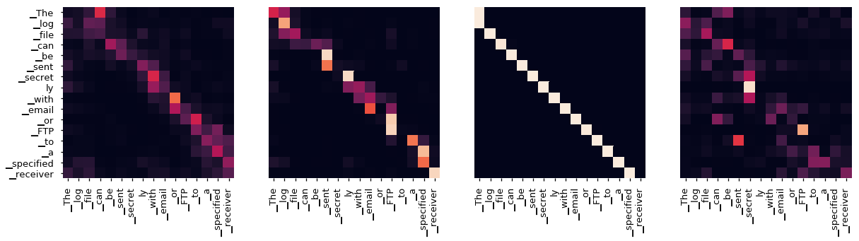encoder_self_attention_harvard Fig. Self-Attention 에 필요한 QK attention map 예시. 원래는 이를 다 저장하고 있어야 함. Source from here

이 paper의 key idea는 이 \(QK^T\)를 다 가지고 있을 필요가 없다는 것이다.

Key Idea

다시 sequence length를 \(L\)이라 하자. 먼저 L개 중에 하나의 token query에 대해서만 생각해 봅시다. 그러면 이 query는 \(d\)차원 밖에 되질 않습니다 \(q \in \mathbb{R}^d\). key, value는 마찬가지로 \(d\)차원의 vector가 n개씩 (\(k_1, \cdots, k_n\), \(v_1, \cdots, v_n\)) 있는것이다. 먼저 standard attention의 경우 아래의 operation을 거치는데,

\[\begin{aligned} & s_i = dot(q, k_i), s'_{i} = \frac{e^{s_i}}{\sum_j e^{s_j}} & \\ & attention(q,k,v) = \sum_i v_i s'_i \\ \end{aligned}\]

이는 다음과 같다.

1.query, \(q\) 하나를 모든 key, \(k_i\)와 각각 내적한다.
- 이 과정에서 \(s_i\) vector가 n개 생김 (space and time complexity 모두 \(O(n)\))
2.softmax로 \(s = (s_1, \cdots, s_n)\) matrix를 row-wise로 normalize한다.
3.normalize된 \(s_i'\)(scalar)와 모든 value, \(v_i'\)를 곱해서 더한다.

이 operation을 모든 n개 token query에 대해서 수행해야 함으로 self-attention의 full space complexity는 \(O(n^2)\)이 되는 것인데, 우선 한 query에 대해서만 생각하자. 이것과 정확하게 같은 (exact same)연산을 memory관점에서 효율적으로 할 수 있는데, 핵심은 우리가 원하는것은 normalize한 score값과 각 value을 곱해서 더하는 weighted sum 이기 때문에 한번에 normalized score를 구하지 않고 아래의 수식처럼 점진적으로 계산 할 수 있다는 것이다.

\[\begin{aligned} & s_i = dot(q, k_i), s'_{i} = \color{red}{e^{s_i}} & \\ & attention(q,k,v) = \frac{\sum_i v_i s'_i}{\color{red}{\sum_j s_j'}} \\ \end{aligned}\]

먼저 \(v^{\ast} \in \mathbb{R}^d\), \(s^{\ast} \in \mathbb{R}^d\)라는 변수를 0으로 initialize 해준다. 그 다음부터는 아래의 과정을 거친다.

1.먼저 \(q\)와 \(k_i\)연산을 \(i=1\)에 대해서만 해준다.
2.그 다음 \(s_i = dot(q,k_i)\)을 계산한다.
3.\(v^{\ast}와 s^{\ast}\)를 각각 \(v^{\ast} \leftarrow v^{\ast} + v_i e^{s_i}\), \(s^{\ast} \leftarrow s^{\ast} + e^{s_i}\)로 update 한다.
1,2,3을 모든 key, value에 대해 반복 (n번)
마지막으로 \(\frac{v^{\ast}}{s^{\ast}}\)로 나눠준다.

Softmax operation을 곱씹어 본다면 이렇게 계산하는것이 standard attention과 완전하게 동치인 것을 알 수 있다. 이러면 사실상 query하나에 대한 space complexity는 scalar하나를 담을 variable만 있으면 이 variable에 이후 모든 token들간의 dot product를 exponential취한 것을 누적해주면 되기 때문에 memory가 더이상 필요하지 않다. 이 연산은 softmax계산을 마지막에 한 번 나누는것으로 처리하기 때문에 lazy softmax라고도 불리기도 하고, 누적해서 연산하기 때문에 cumulative normalized attention score라고도 한다. 대신에 query를 먼저 읽고 key, value pair의 list가 특정 order에 맞게 들어와야하는 문제가 있어 만약 그 순서대로 들어오지 않는다면 이를 정렬하기 위한 index에 대한 정보를 가지고 있어야 하므로 \(O(\log n)\)만큼이 필요하다고 한다.

당연하게도 이를 모든 query에 대해 계산하는 self-attention으로 확장할 수 있고, query들에 대한 index를 위해 \(O(\log n)\)이 필요하고 \(O(n)\)의 outputs이 만들어집니다.

attention: \(O(1)\)
self-attention: \(O(\log n)\)

Numerical Stability

그런데 원래 torch나 tensorflow에서는 softmax를 계산할 때 numerical stability를 위해서 어떤 장치를 해두는데 지금은 torch.nn.functional.softmax를 쓰는 것이 아니라 manually softmax를 해준것이나 다름이 없기 때문에 이 처리를 따로 해줘야 한다. 이 trick을 해줘야 하는 이유는 softmax를 취하는 것이 element들을 exponential 취하는데 이 값이 89를 넘어가면 float16은 말할 것도 없고 float32이나 bfloat16에서 inf값을 return하기 때문이다. 그래서 softmax를 취할 때는 보통 그 element들 중에서 가장 큰 값을 빼주는데 이렇게해도 softmax normalized score의 결과는 바뀌지 않기 때문에 이를 활용하는 것이다.

\[attention(q,k,v) = \frac{\sum_i v_i e^{s_i \color{red}{-m}}}{\sum_j e^{s_j \color{red}{-m}}} = \frac{\sum_i v_i e^{s_i} \color{red}{e^{-m}}}{\sum_j e^{s_j}\color{red}{e^{-m}}}\]

결과적으로 \(v^{\ast},s^{\ast}\)에 이어 \(m^{\ast}\)를 하나 더 관리해야 하는데, 이는 \(m^{\ast}=-inf\)로 초기화 한다. 그리고 q,k를 계산해서 score, \(s_i\)를 만든 뒤에 먼저 \(m_i = max(m^{\ast}, s_i)\)를 해주고 각 update 수식들을 아래처럼 numerical stable하게 memory efficient SDPA를 구현하는 것이 된다.

1.\(v^{\ast} \leftarrow v^{\ast} \color{red}{e^{m^{\ast}-m_i}} + v_i e^{s_i-\color{red}{m_i}}\)
2.\(s^{\ast} \leftarrow s^{\ast} \color{red}{e^{m^{\ast}-m_i}} + e^{s_i-\color{red}{m_i}}\)
3.\(m^{\ast} \leftarrow m_i\)

Chunk-wise Operation (for parallelism)

그 다음으로 위의 idea를 실제로 구현할 때 중요한 사항이다. 앞서 언급한 algorithm을 그대로 갖다 쓰는것은 실제로 매우 느릴 수 있는데 (병렬화 하기가 어려움) 왜냐하면 score, weighted value값을 1개씩 누적시키면서 계산하기 때문이다. 그래서 query, key, value pair를 chunk단위로 나눠서 누적하는 방법을 쓸 수 있는데, 이러면 memory efficiency가 조금 떨어지지만 속도가 조금 빨라질 것이다. (명심해야 할 것은 언제나 speed와 memory, 이 둘은 trade-off가 있다는 것이다.)

xformers_chunk Fig. query쪽 chunk size와 , key-value의 chunk size는 다르다. SDPA의 output을 보면 query size만한 하나의 output chunk를 만들기 위해서 for loop을 돈다는 것을 알 수 있다. for loop을 돌면서 누적시키는 것이 앞서 소개한 기술이며, 여기서 q@k를 하는 것은 chunk size가 query는 x이고 key,value는 y라면 원래 대로 \(O(xy)\)이다. Source from xFormers: Building Blocks for Efficient Transformers at PyTorch Conference 2022

위의 animation을 보시면 직관적으로 idea를 이해할 수 있을것인데, 이를 q, k, v를 마치 일정 크기의 타일 (tile)로 나눈다고 해서 tiling이라고하며 이는 CUDA kernel을 짤 때 자주 쓰이는 개념이라고 하는 것 같다.

먼저 tiling을 위해 n개의 query, key, value들을 constant chunk size로 split 해야 한다. 그리고 loop을 돌면서 self-attention 연산을 수행할 건데 tile size는 일반적으로 \(\sqrt{n}\)로 정한다 (\(n=1\)이면 위에서 얘기했던 extreme cumulative sum이 recover된다). 그러면 \(n\)개의 key, value들이 (딱 나눠떨어진다는 가정하에) 각각 \(\sqrt{n}\)크기 \(\sqrt{n}\)개로 나눠지게 된다. toy example로 batch_size=4, n=2048, num_head=8, dim=748의 경우를 생각 해보자. 그리고 query_chunk_size=1024로 하고 key_chunk_size=int(math.sqrt(2048))=45라고 하자. (딱 나눠떨어지지않았으므로 key, value chunk size는 45임. query chunk size는 1024)

query.size() torch.Size([4, 1024, 8, 96])
key.size() torch.Size([4, 45, 8, 96])
value.size() torch.Size([4, 45, 8, 96])

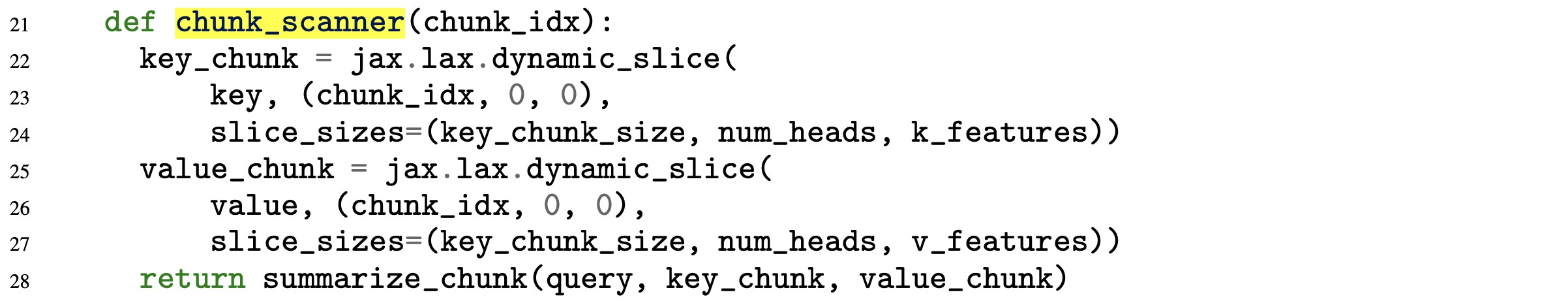
이제 각 query chunk 개수만큼 loop를 돌면서 (inner-loop) self-attention을 하는데, 주어진 query chunk에 대해서 key, value도 loop을 돌면서 (outer-loop) 결과값을 merge한다. 이 때 figure의 caption에 설명한 것 처럼 q@k는 standard attention 처럼 계산한다 (memory cost가 좀 들어감).

# q@k 결과물
attn_weights.size() torch.Size([4, 1024, 8, 45])

그리고 \(s^{\ast}, v^{\ast}, m^{\ast}\)에 해당하는 summaries를 각 chunk 별로 return한다.

mem_efficient_paper_fig1_sub1

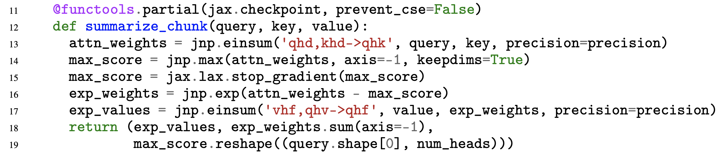
그러면 아래와 같은 \(s^{\ast}, v^{\ast}, m^{\ast}\) summary들이 생기는데,

exp_values.size() torch.Size([4, 1024, 8, 96])
exp_weights.size() torch.Size([4, 1024, 8, 45])
max_score.size() torch.Size([4, 1024, 8])

이를 \(\sqrt{n}\)번 반복하면 summary들이 \(\sqrt{n}\)개가 생길 것이다.

mem_efficient_paper_fig1_sub2

최종적으로 이들을 위에서 말한 것처럼 rescale해주고 merge를 하고 (\(\color{red}{ \sum_{i=1}^{\sqrt{n}}} v_i^{\ast}\), \(\color{red}{ \sum_{i=1}^{\sqrt{n}}} s_i^{\ast}\)), merge된 score값과 value값을 하던대로 나눠주면 된다.

mem_efficient_paper_fig1_sub3

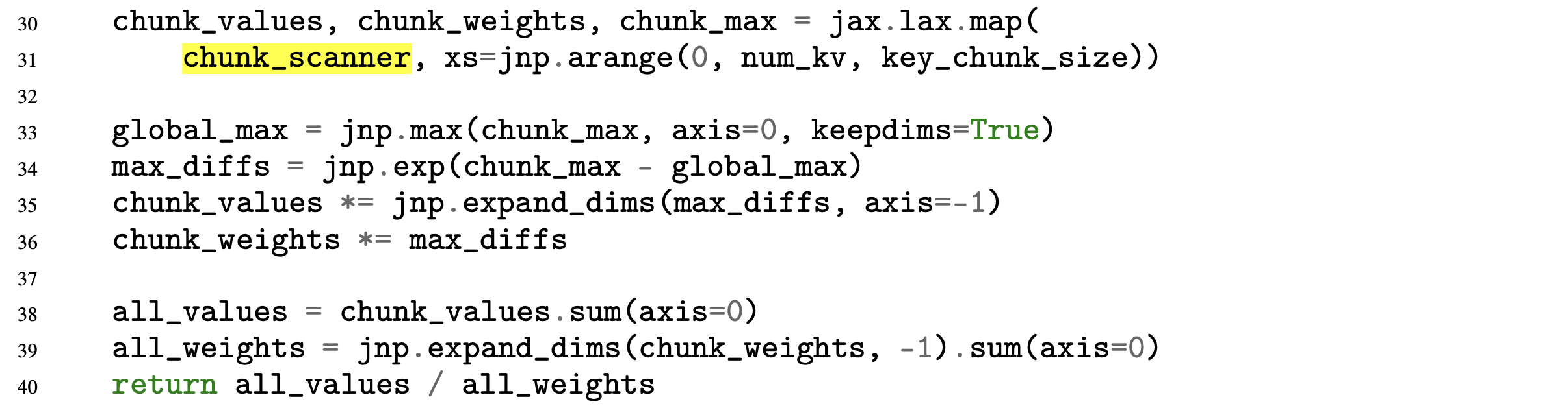
그러니 한 query chunk 기준으로 key, value pair chunk들을 slide 할 때 필요한 peak memory는 q@k에 필요한 memory와 이를 summary할 elements들 까지 해서 \(O(\sqrt{n})\)이 추가로 필요하게 될 것이다. 이렇게 해도 되는 이유는 key, value의 sequence length를 짧은 갯수로 나누기 때문에 그렇게 큰 memory inefficiency는 생기지 않아서 인 것으로 보인다.

attention: \(O(1)\)
self-attention: \(O(\log n)\)
practical self-attention: \(\color{red}{O(\sqrt{n})}\)

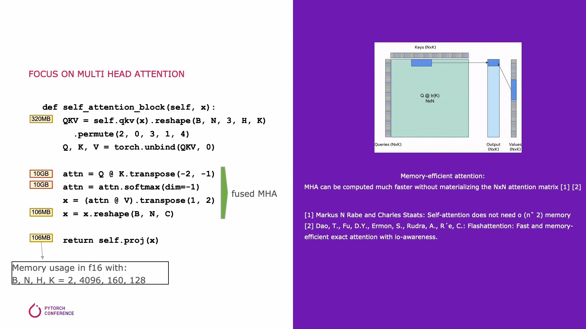before_xformers Fig. xformers를 적용하기 전에는 sequence length N이 4096일 경우 10GB가 필요하다.

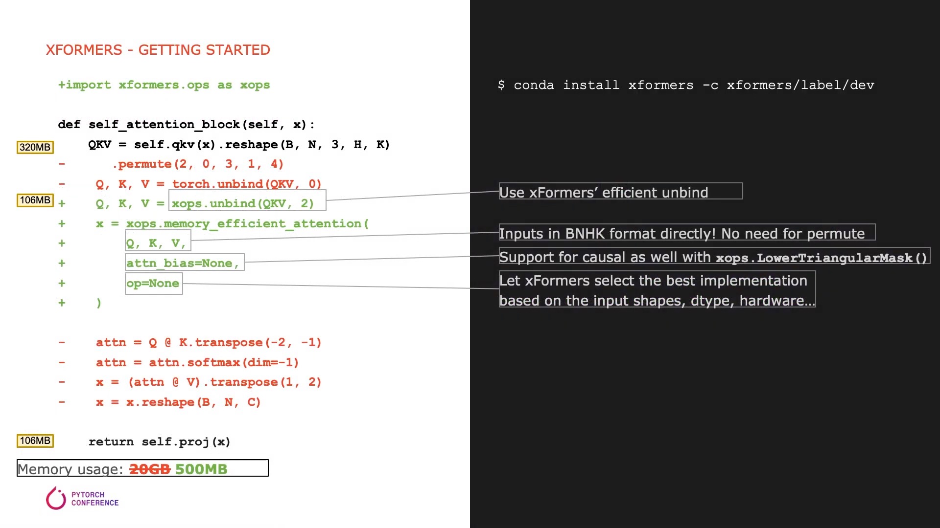after_xformers Fig. xformers를 적용한 후에는 (kernel fusion이 추가적으로 들어가긴 했으나) 106MB로 줄어든다. (kernel fusion은 추후에 설명)

Inference Results

이렇게 최적화를 하면 self-attention에 대해서 input sequence의 길이를 바꿔가면서 inference해봤을 때 모든 구간에서 상당한 개선이 있었음을 알 수 있다. 특히나 길이가 \(n > 2^{16}\)인 경우에 대해서는 OOM (Out of Memory)이 나던것이 나지 않게 되었다.

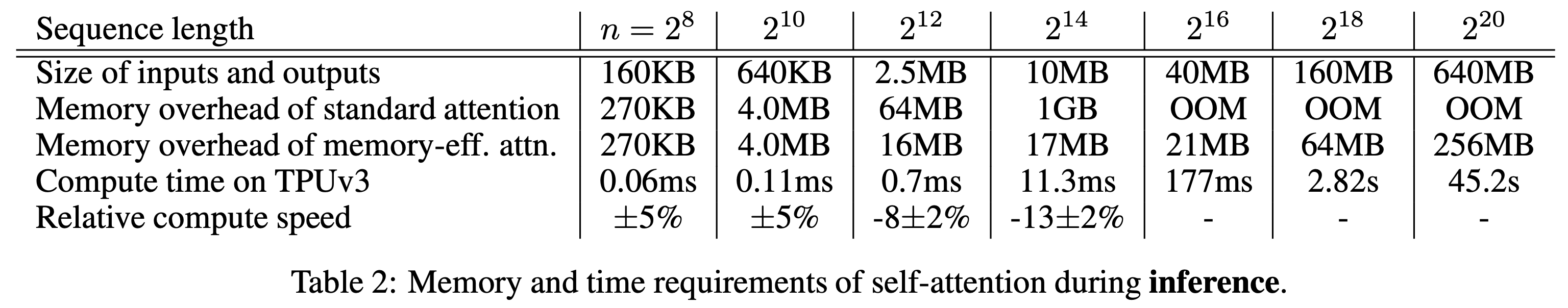mem_efficient_paper_table2 Fig.

TPU에서 연산했고 SDPA의 input의 경우 bf16 precision이니 2bytes지만 attention 계산을 할 때부터는 fp32를 써서 4bytes로 계산해야 하는데, 위의 table 결과는 peak memory를 측정한 것이라고 해서 정확히 어떻게 위의 값들이 계산 되었는지는 정확하게 알지는 못하겠어서 넘어가도록 하겠다. 어쨌든 \(n < 2^{10}\)인 경우에 대해서는 query, key chunking을 하지 않았으므로 (query_chunk_size=1024, key_chunk_size=4096이 default인데 이 값을 사용한듯?) 큰 차이가 발생하지 않은것으로 보이고, 그 이상의 경우에는 속도가 조금 유의미하게 감소한 것 같다.

이러한 실험 결과는 self-attention 만을 대상으로 한 것이기 때문에 Transformer 전체로 확장하게 되면 model내에 FFN이나 다른 요소들도 있을 것이기 때문에 self-attention operation의 비중이 줄어들어 조금 상이한 결과가 나올 수도 있음에 주의해야 한다. (실제로 실험해보면 이론상의 improvement는 없을 수 있음)

논문의 abstract을 보면 16384 길이의 input에 대해서 inference에서는 59배나 memory overhead를 줄였다고 언급이 되어있다.

For sequence length 16384, 
the memory overhead of self-attention is reduced by 59X for inference 
and by 32X for differentiation.

Differentiation

Forward는 속도는 조금 손해봤지만 memory를 많이 아꼈다고 치자. 그런데 학습에도 이를 적용하려면 softmax를 위한 \(s_i'\)등의 중간 결과 (intermediate result)들을 다 들고 있어야 backpropagation을 할 수 있기 때문에 문제가 발생한다. 그러니까 어차피 다 어딘가에 저장하고 있으면 순차적으로 \(v^{\ast}, s^{\ast}\)에 누적시켜가며 계산을 하는 것이 어떠한 이점도 줄 수 없는 것이다. 이를 해결하기 위해서 저자들은 gradient (activation) checkpointing과 유사한 technique을 제안했다 (그냥 gradient checkpointing이라고 보면 된다). Gradient checkpointing은 간단하게 말하자마녀 터무니 없이 큰 모델을 학습할 때 layer들의 activation output들을 다 저장하지 않고 일부만 띄엄 띄엄 저장한 다음에 forward가 다 끝나면 loss를 계산하고 backpropagation을 할 때 빈 activation output들을 다시 계산 (recomputation)하는 trick을 말한다. 아래의 animation을 보시면 vanilla backpropagation을 할 경우, forward activation을 다 저장해 둔 다음에 끝에가서 loss를 계산하고 차례 차례 memory를 release하는 걸 보실 수 있다.

vanilla_backprop Fig. Vanilla Backprop

만약 GPU에 memory를 model 올리는 데 이미 거의 다 썼다면 아래와 같이 정말 비효율적으로 다시 계산하는 방법을 택할 수 도 있을 것이다.

memory_poor_backprop Fig. Memory Poor Backprop

Activation checkpointing은 이 둘의 절충안으로 checkpoint지점들을 두고 그 지점부터만 현재 node까지 빈 activation을 다시 계산하는 식으로 구현된다.

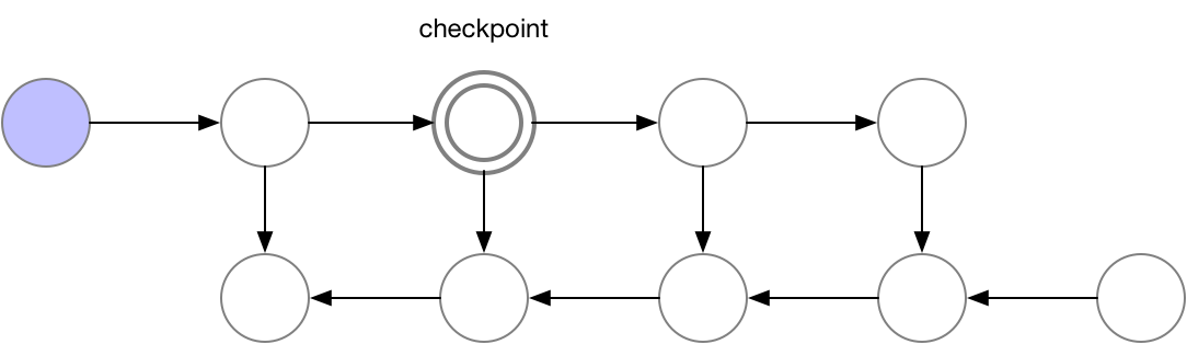checkpointed_backprop Fig. Checkpoint of Activation Checkpointing method

checkpointed_backprop Fig. Checkpointed Backprop

이 과정이 paper의 implementation code에도 아래와 같이 구현이 되어 있다. (chunk별 summary를 별도로 저장하고 있음)

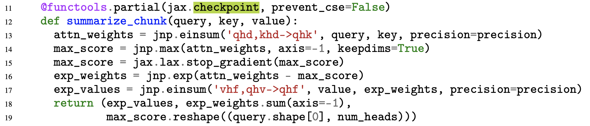
mem_efficient_paper_fig1_checkpoint

이 trick을 vanilla attention에도 적용하면 되지 않을까?라는 생각이 들 수도 있지만 저자들은 이점이 없을것이라고 한다. 왜냐면 vanilla attention은 어찌됐든 full attention score map을 생성한 다음에 지우는 것이 되기 때문이다. 어쨌든 미분을 하는 과정에서의 time and space complexity를 측정했을 때 seuqnece length가 길어질수록 memory관점에서는 매우 효율적이지만 re-computation 때문에 조금은 느려지는 걸 감수해야 한다.

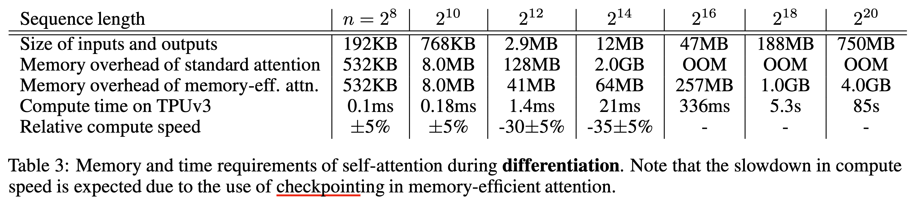mem_efficient_paper_table3 Fig.

Comparison of Training Performance between Vanilla and Memory Efficient Attention

실제로 학습에 나쁜영향을 미치지 않는지 궁금한 사람이 있을것이다. 이론적으로는 exact same이기 때문에 별 차이가 없어야 하지만 computer라는 것이 본래 operation 순서만 바뀌어도 결과가 바뀌는 것이기 때문에 문제가 생길 여지가 있다. Paper에서는 SDPA를 다르게 썼을 때 machine translation dataset으로 transformer를 학습해 BLEU score 를 비교해 봄으로써 둘 사이에 큰 차이가 없었음을 밝혀냈다.

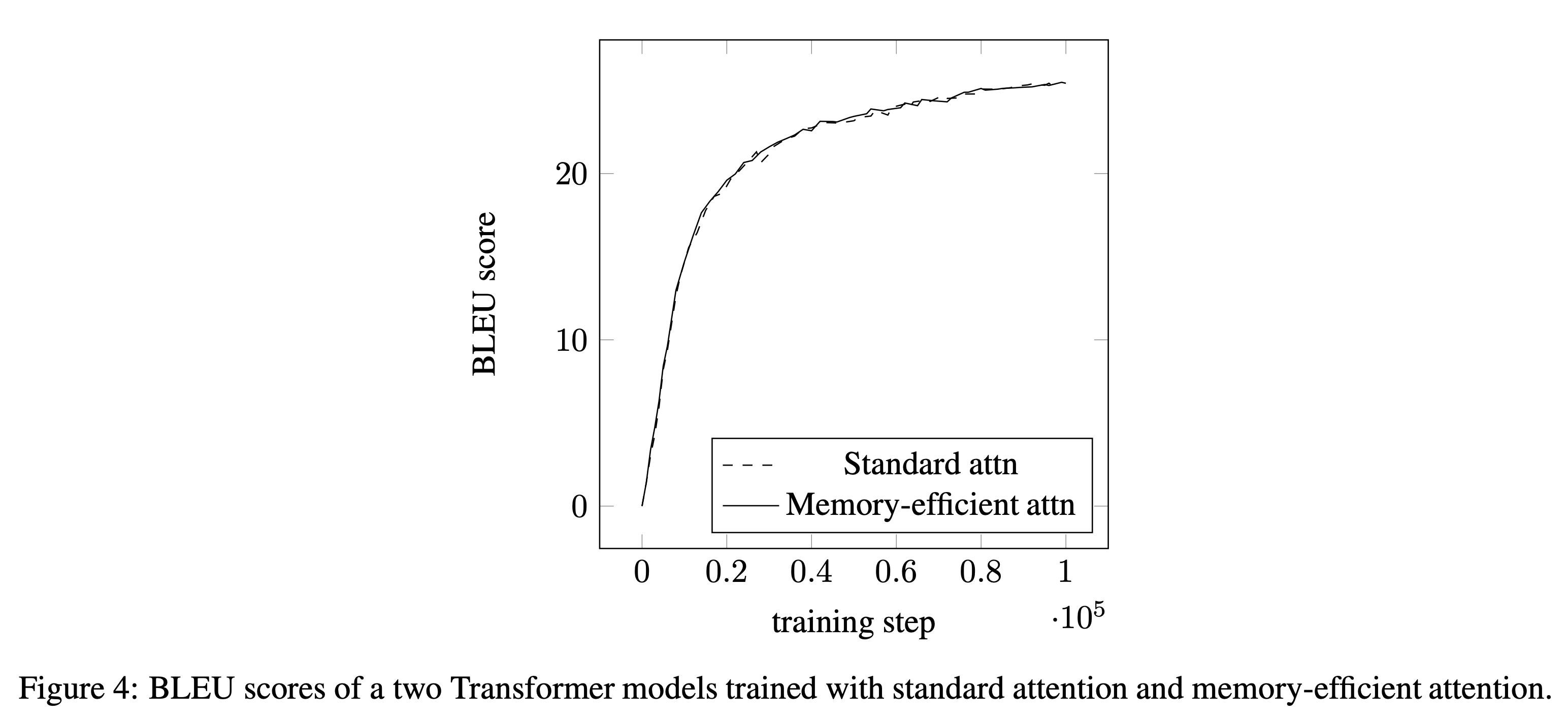mem_efficient_paper_fig4 Fig.

Memory efficient attention은 이렇듯 간단한 trick만으로 memory cost를 어마어마하게 개선했는데, 마지막 related work section에는 이런 말이 있다.

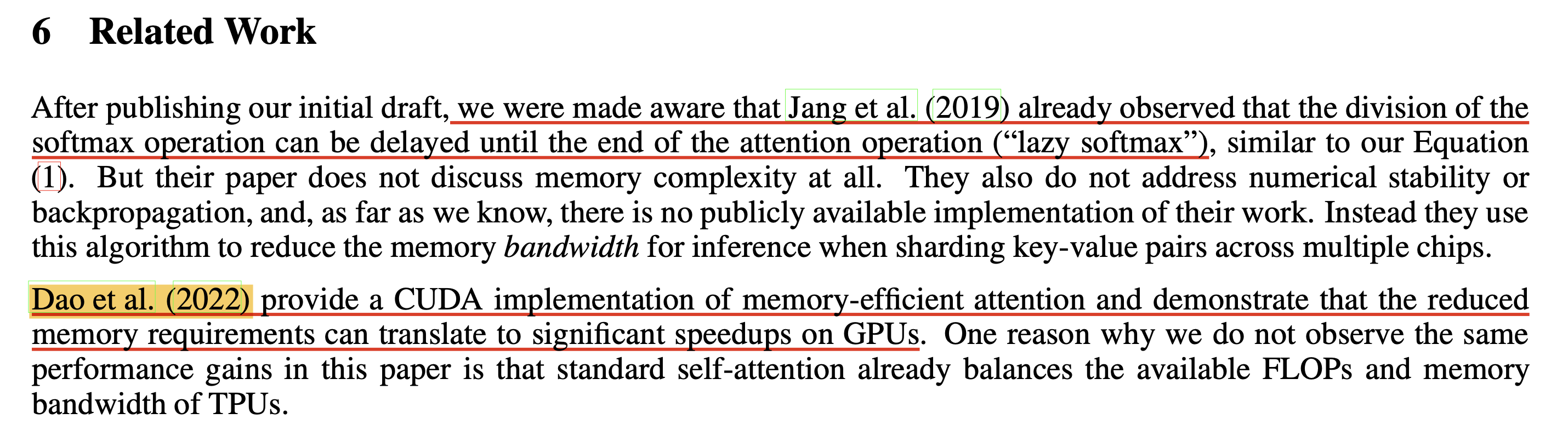mem_efficient_paper_last_phrase Fig.

뭐 당연히 Transformer 최적화 관점에서 고민하던 연구자들이 많았을테고 유사한 방법론은 어떤게 있으며 자기들은 이런 차이가 있다 하는 말들과 함께 마지막에 Dao et al.을 언급하는데, 자신들의 work을 CUDA version으로 구현함으로써 속도개선까지 이뤄낸 related work이 있다는 것이다. 그리고 그것이 바로 Flash Attention이다.

Flash Attention

FlashAttention: Fast and Memory-Efficient Exact Attention with IO-Awareness는 Stanford 연구진이 발표한 논문이다. (1저자는 2023년에 Princeton University 에서 조교수로 임용이 됐고 2023년 7월 현재는 FlashAttention-2: Faster Attention with Better Parallelism and Work Partitioning까지 나왔다)

앞서 말했다시피 memory efficient하게 cumulative normalized attention score를 구하는 것은 기본이고, A100 GPU의 특성까지 살려서 속도 개선까지 해서 사실상 요즘 나오고있는 모든 optimized training, inference library에는 기본적으로 들어가는 module이 됐다. 아래 table 2를 보면 autoregressive manner로 학습되는 GPT-2 Language Modeling (LM) task에서 huggingface (vanilla attention을 쓴 것) 대비 training time을 3.5배나 save한 것을 볼 수 있다.

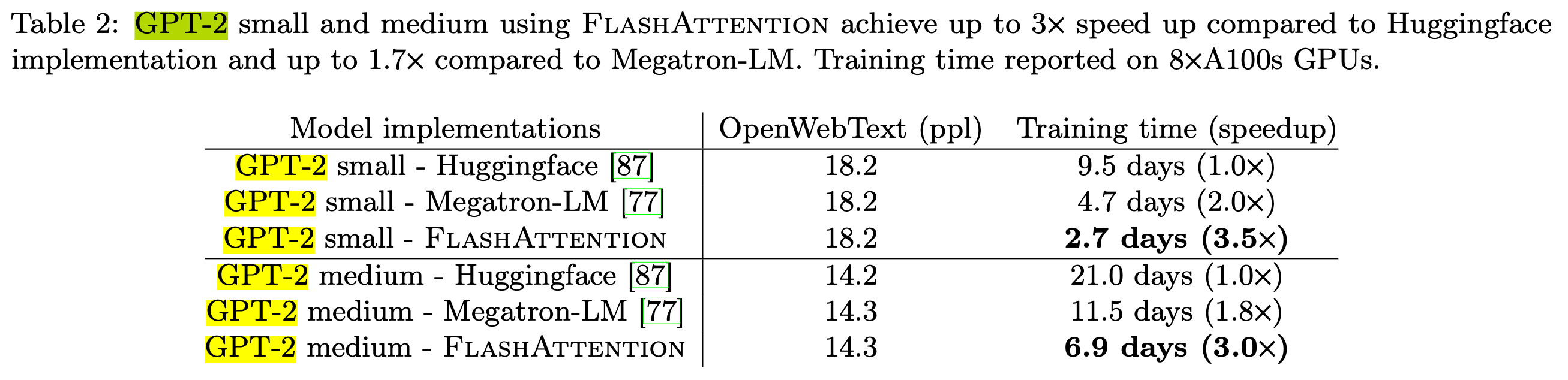flash_attn_v1_paper_table2 Fig.

이제 Flash Attention 에 대해서 간단하게 알아보자.

Key Idea (Reduced IO Complexity + Tiling)

Flash attention의 철학을 이해하기 위해서는 GPU라는 hardware의 hierachy와 performance characteristic을 알아야 한다. 보통 어떤 operation을 수행하는 것 자체는 실제 연산을 수행하는 것 (computation)과 SRAM, HBM 등 memory에 접근하는 것 (memory access)의 balance에 따라서 compute bound와 memory bound로 분류되는데, 이는 다음과 같다.

Compute-bound : 얼마나 많은 arithmetic operation을 하는가? 에 따라서 전체 operation의 time이 정해짐.
- 주로 큰 inner dimension을 갖는 matrix multiplication (matmul)이거나 channel수가 많은 convolution 등이 이에 해당됨
Memory-bound : Memory access에 따라 operation의 time이 정해진다.
- elementwise (e.g. activation, dropout) 이나 reduction (e.g. sum, softmax, batch norm, layer norm) 등이 이에 해당됨

flash_attn_v1_paper_fig1_sub1 Fig.

flash_attn_v1_paper_fig1_sub2 Fig.

flash_attn_v1_paper_fig1_sub3 Fig.

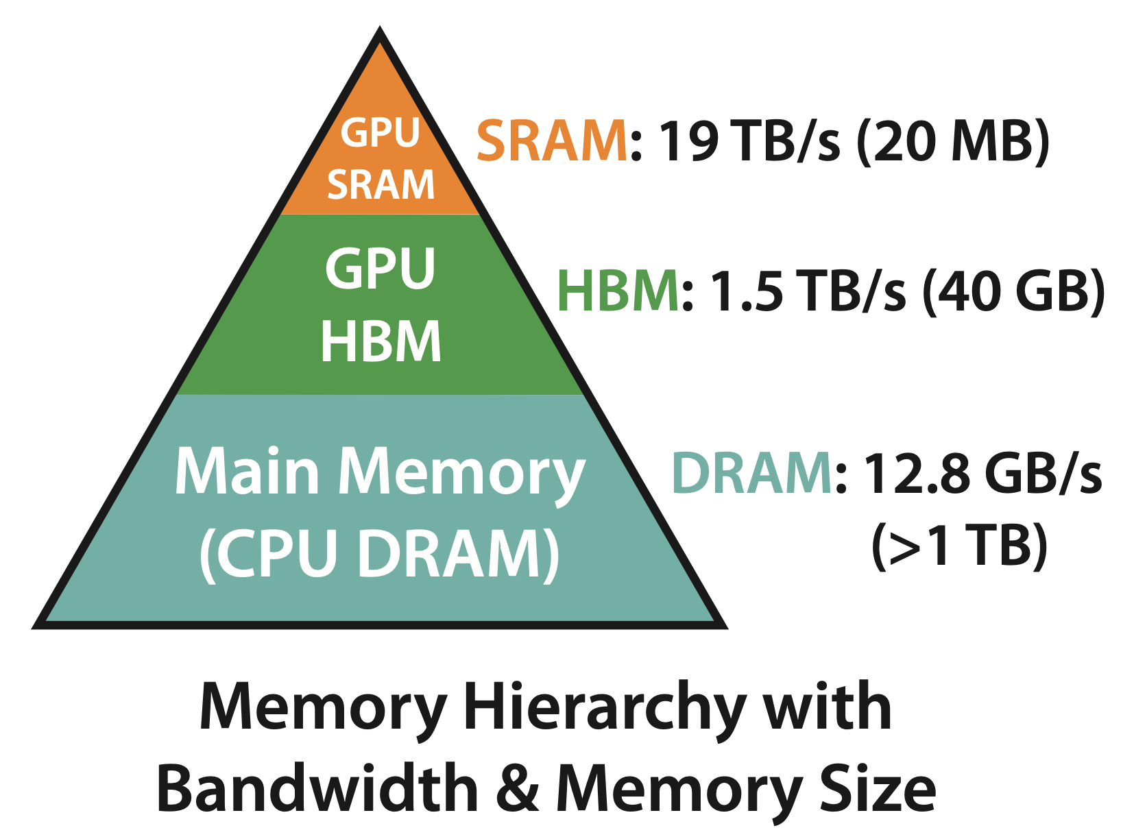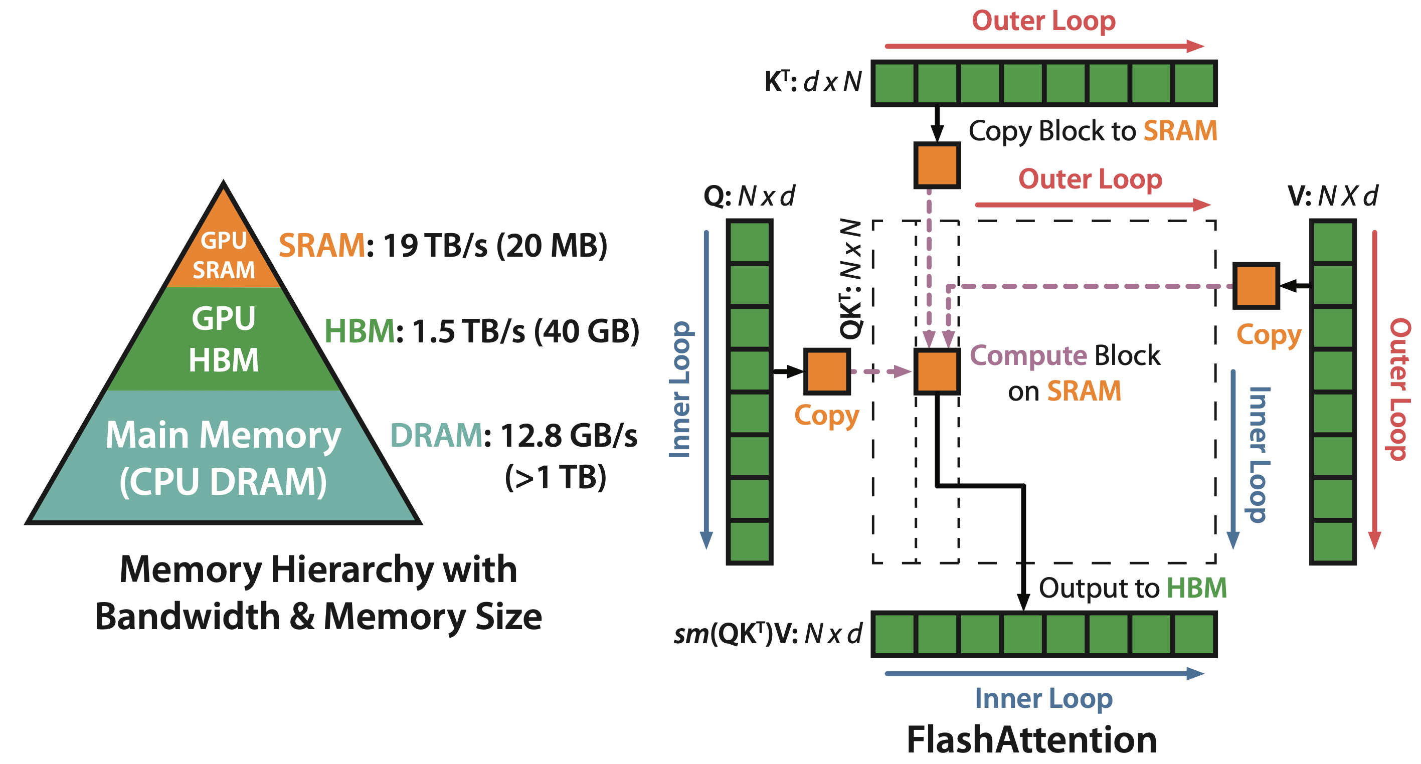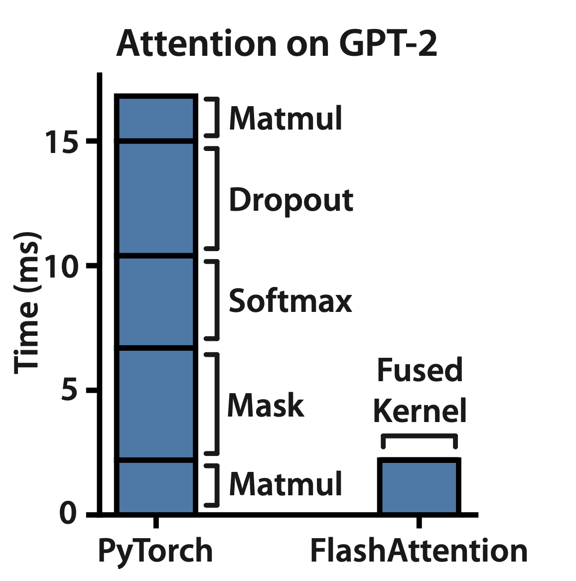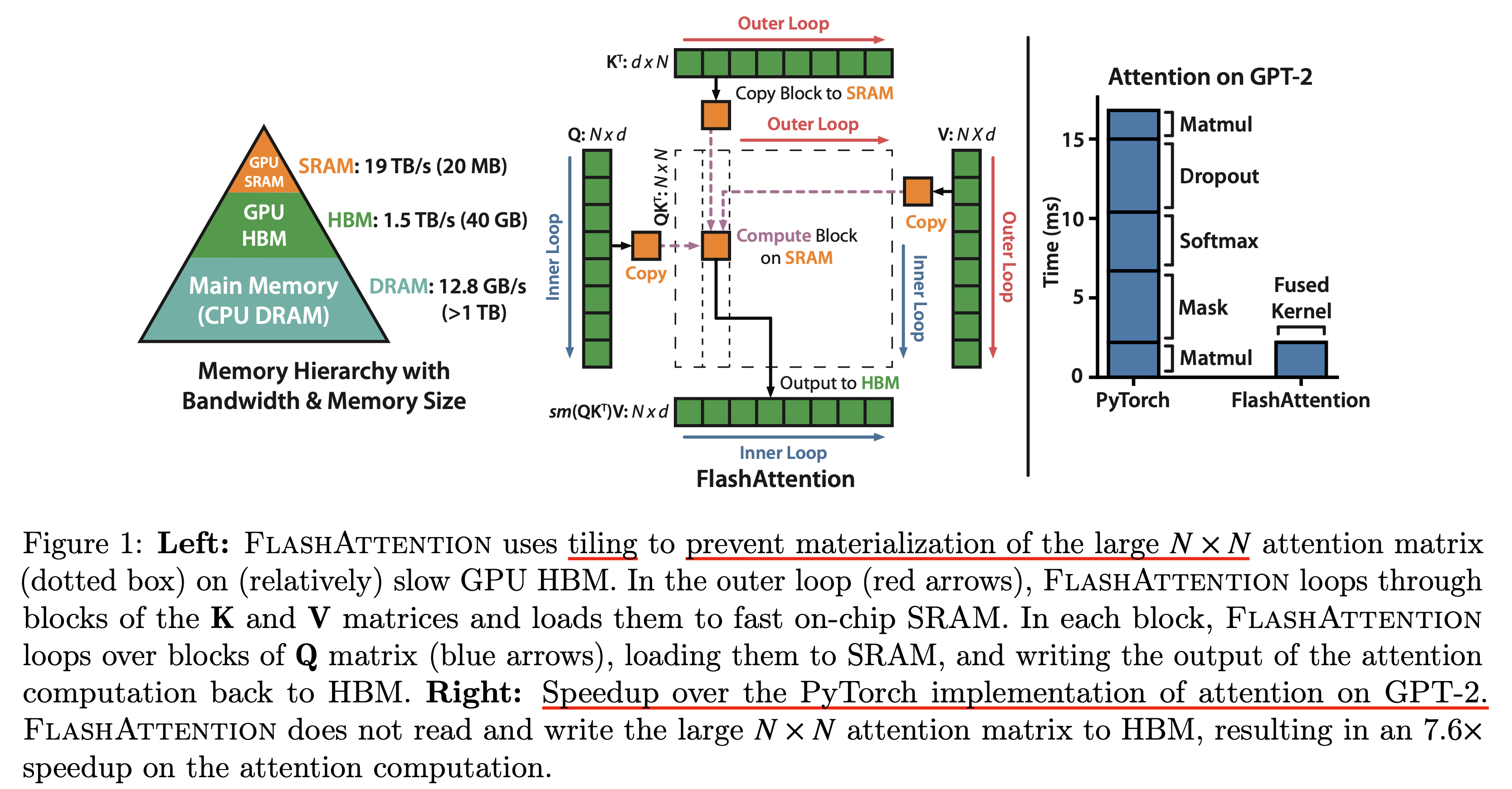flash_attn_v1_paper_fig1 Fig. Overview of Flash Attention version 1

flash attention의 전체 algorithm을 알아보기 전에 standard attention의 algorithm을 먼저 보자.

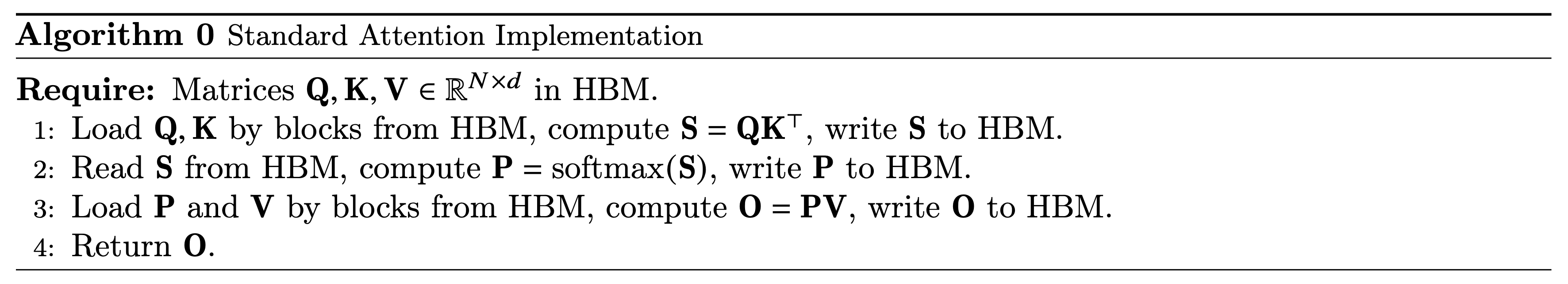flash_attn_v1_paper_algorithm0 Fig.

Standard attention의 경우 batch를 제외하고 (batch가 1인) \(Q,K,V \in \mathbb{R}^{N \times d}\)의 matrix가 있다고 쳤을 때, attention output matrix, \(O \in \mathbb{R}^{N \times d}\)를 구하기 위해서 \(Q,K\)를 HBM으로부터 불러온 다음 matrix multiplication을 통해 \(S=QK^T\)를 계산해서 얻은 output을 다시 HBM에 저장해야한다. 그리고 score map을 softmax로 normalize하기 위해서 다시 HBM으로부터 \(S\)를 읽어 \(P=softmax(S)\)를 해 HBM에 \(P\)를 저장한 뒤, 마지막으로 다시 \(P,V\)를 HBM 에서 읽은 뒤 \(O=PV\)를 계산하여 이 결과를 HBM에 저장한다.

결과적으로 HBM의 read/write (Input/Output; I/O)가 발생하는데 이럴 필요가 없다.

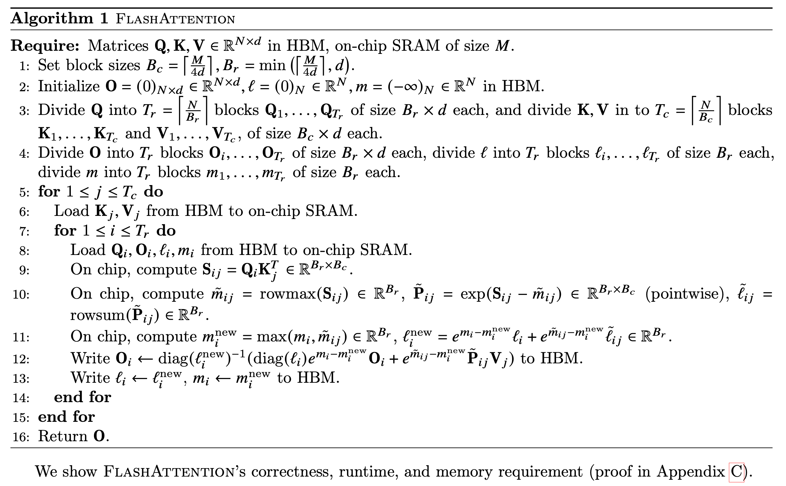flash_attn_v1_paper_algorithm1 Fig.

Flash attention은 아래의 theorm에 따라 \(O(N^2 d)\)의 연산량 (FLOPs)를 가지며 이는 \(O(N)\)의 추가적인 memory를 필요로 한다.

flash_attn_v1_paper_theorm1 Fig.

이제 flash attention의 I/O complexity에 얼마나 개선이 있었는지 분석해보자. Flash는 tiling을 통해서 space complexity를 줄였지만 그만큼 backward시 recomputation해야 하기 때문에 time complexity가 증가한다. 하지만 flash attention은 SRAM size가 \(M (\text{ where } d \leq M \leq Nd)\)일 때 \(O(N^2 d^2 M^{-1})\)의 HBM access가 필요하지만, 이 수치는 SRAM size가 클수록 discount되기 때문에 standard attention은 \(O(Nd + N^2)\)보다 훨씬 작다.

flash_attn_v1_paper_theorm2 Fig.

그러므로 recomputation때문에 실제 연산량 (FLOPs)가 늘어나는 문제가 있어도 충분히 cover가 되고도 남는다. 즉 A100같은 architecture에서 flash는 space, time complexity를 모두 해결한 것이 되는 것이다. 이는 당연하게도 sequence length, \(N\)이 증가할수록 더 차이가 날 것이며, 아래 figure는 이를 설명하는 table과 plot이다.

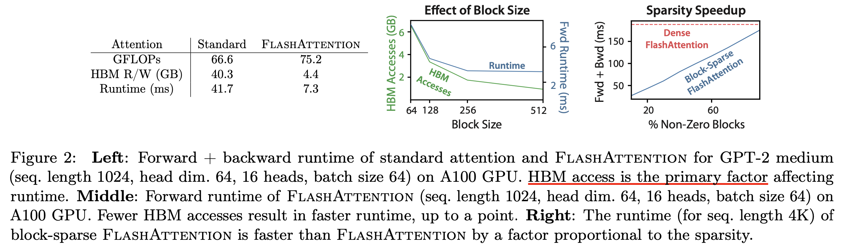flash_attn_v1_paper_fig2 Fig. (중간) block size가 커질수록 HBM access에 드는 complexity가 줄어들지만 어느순간 runtime이 더이상 줄어들지 않는다. Block Sparse Attention은 지금 다루지 않는다.

Forward Pass Details

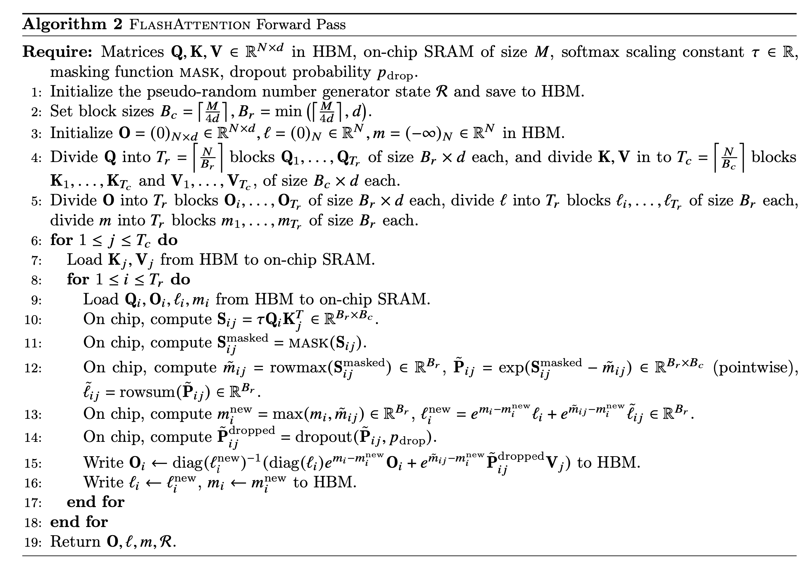flash_attn_v1_paper_algorithm2 Fig.

Backward Pass Details

flash_attn_v1_paper_algorithm3 Fig.

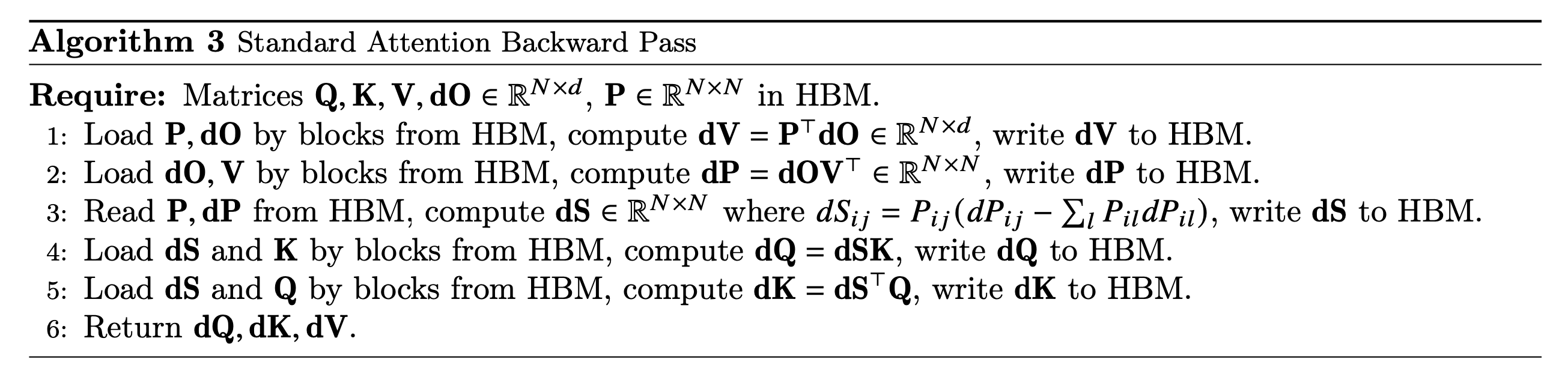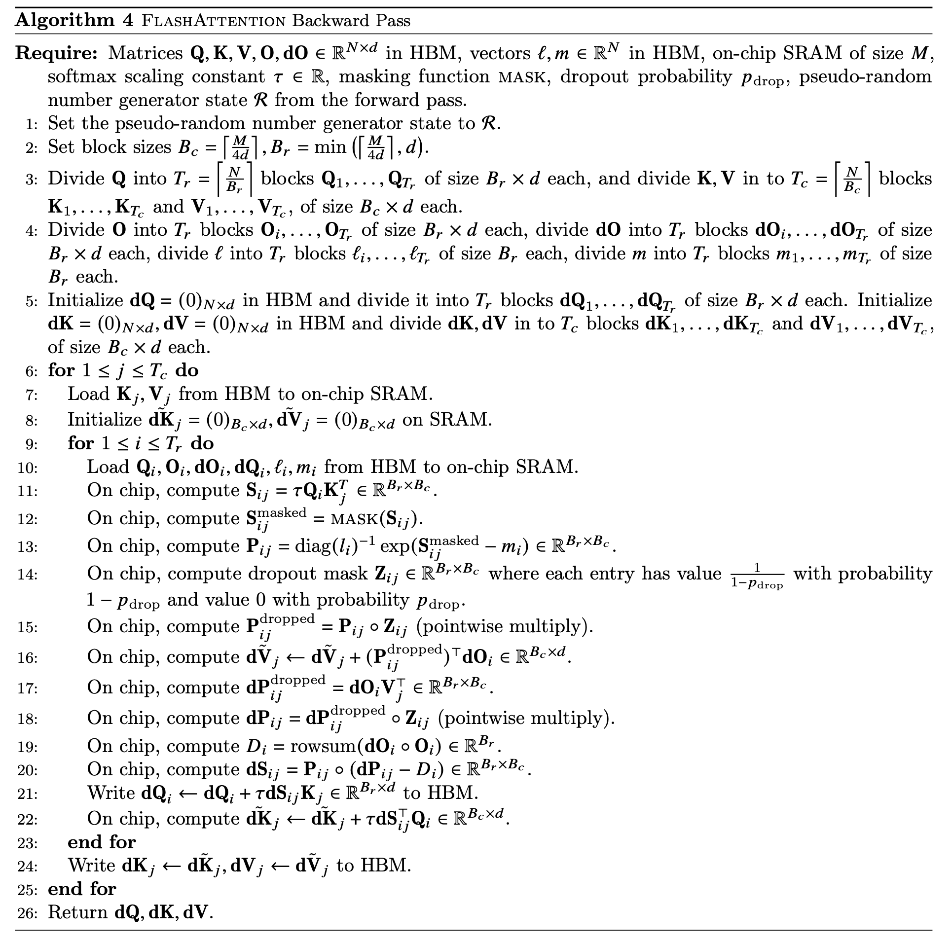flash_attn_v1_paper_algorithm4 Fig.

그러나 backward pass는 atomic adds를 사용하기 때문에 non-deterministic하다고 한다 (issue 참고).

Compared to Staats et al.

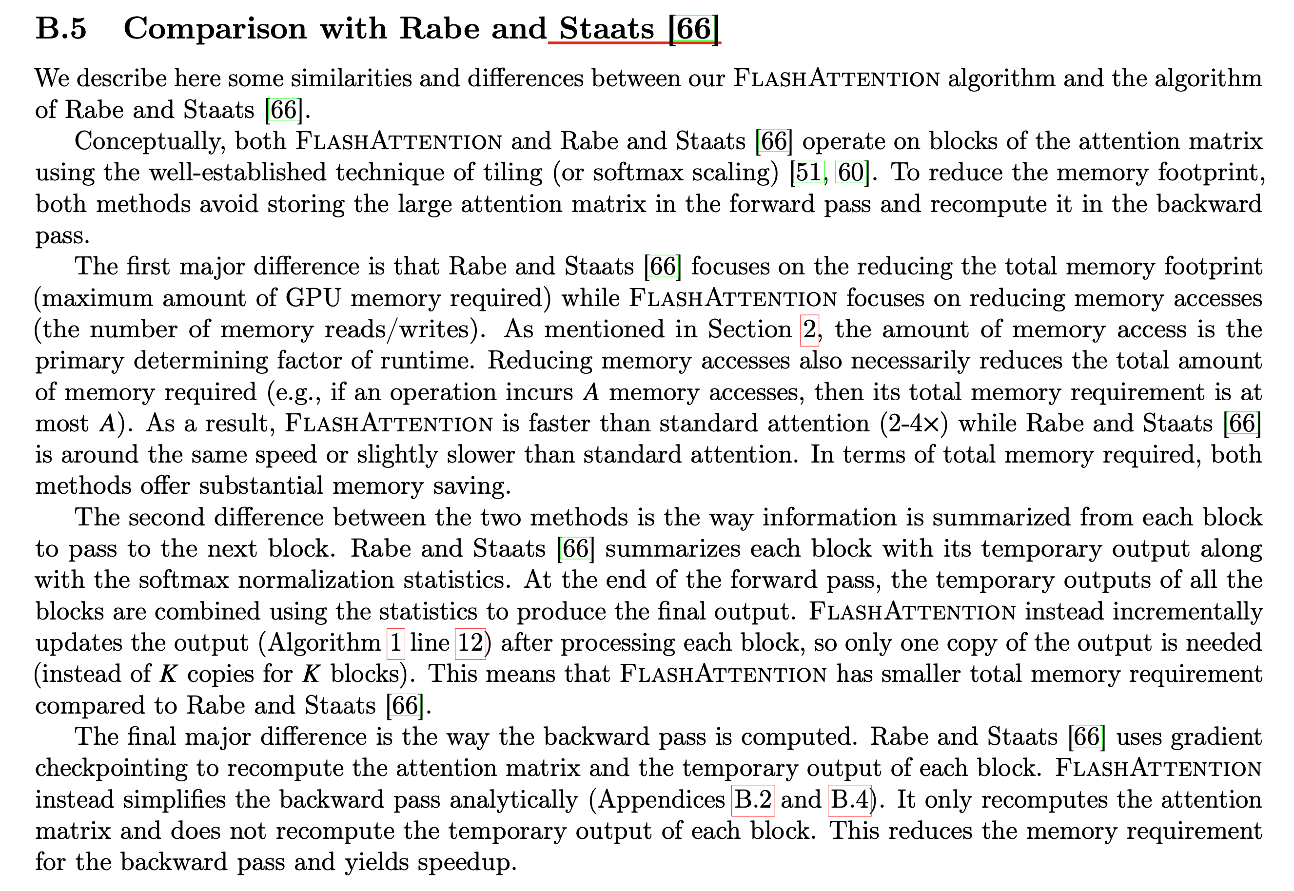flash_attn_vs_xformers Fig.

Implementation of Efficient SDPA

Torch Built-in SDPA

Flash attention 등 efficient SDPA를 사용하기위한 방법은 크게 아래 세 가지가 있다.

Official repo for FlashAttention
xformers
torch 2.0.0 이상 version

사실 이 세개가 거의 같은 kernel을 쓰기 때문에 뭘 써도 무방하지만 개인적으로 xformers를 추천한다. xformers는 이름답게 transformer에 도움이되는 module은 다 때려박은 것으로 meta에서 만든 library인데, 이미 flash attention의 모든 kernel이 들어가 있다. 그리고 pytorch도 마찬가지로 meta의 framework이기 때문에 xfomers에서 검증이 되면 (stable 해지면) torch로 넘어온다. 즉 xformers를 쓰는것이 가장 빠르다고 할 수 있다.

Pytorch 에서는 Transformer 의 bottleneck 중 하나인 SDPA 연산을 효율적으로 하기 위해서 자체 제작한 kernel을 도입한 Transformer 를 torch.nn 에서 사용할 수 있게 update해왔다. torch.nn.MultiheadAttention나 torch.nn.TransformerEncoderLayer 구현체 내에는 F.multi_head_attention_forward 라는 c++ 로 구현된 구현체를 사용해서 multi head attention 연산을 사용하는데, 이 함수에는 torch._C._nn.scaled_dot_product_attention 라는 SDPA 구현체를 쓰며 이는 torch version이 update 수록 더 개선이 되어 왔다. Torch 2.0 이상부터는 F.scaled_dot_product_attention 라는 함수를 torch.nn.functional 로 부터 call 할수 있게 되었는데, 앞서 설명한 것 처럼 이 function이 효율적인 이유는 크게 세 가지다.

A PyTorch implementation defined in C++
FlashAttention : Fast and Memory-Efficient Exact Attention with IO-Awareness
xformers : Memory-Efficient Attention

Cpp로 짜여졌으므로 좀 더 빠르고 나머지는 flash attention 에서 사용한 tiling과 fused kernel 얘기다.

Using F.scaled_dot_product_attention

그럼 naive implementation 과 torch sdpa 가 얼마나 차이가 나는지 비교해보자. 먼저 naive attention을 계산해보자.

import math
import tqdm

import torch
import torch.nn as nn
import torch.nn.functional as F

device = "cuda" if torch.cuda.is_available() else "cpu"

bsz = 4
n_head = 8
n_feat = 768
seq_len = 100

d_k = n_feat // n_head

linear_q = nn.Linear(n_feat, n_feat).to(device)
linear_k = nn.Linear(n_feat, n_feat).to(device)
linear_v = nn.Linear(n_feat, n_feat).to(device)
linear_out = nn.Linear(n_feat, n_feat).to(device)

x = torch.rand(bsz, seq_len, n_feat, device=device) # B, T, C

q = linear_q(x).view(bsz, -1, n_head, d_k).transpose(1, 2) # B, H, T, C
k = linear_k(x).view(bsz, -1, n_head, d_k).transpose(1, 2) # B, H, T, C
v = linear_v(x).view(bsz, -1, n_head, d_k).transpose(1, 2) # B, H, T, C

def forward_attention(q, k, v, bsz, n_head, d_k):
    attn_weight = torch.softmax(q @ k.transpose(-2, -1) / math.sqrt(q.size(-1)), dim=-1)
    out = (attn_weight @ v)
    return out.transpose(1, 2).contiguous().view(bsz, -1, n_head * d_k)

out = forward_attention(q, k, v, bsz, n_head, d_k)
out1 = linear_out(out)

아래처럼 바꿔주면 되는거죠.

def forward_efficient_sdpa(q, k, v, bsz, n_head, d_k):
    out = F.scaled_dot_product_attention(q, k, v)
    return out.transpose(1, 2).contiguous().view(bsz, -1, n_head * d_k)

out = forward_efficient_sdpa(q, k, v, bsz, n_head, d_k)
out2 = linear_out(out)

실제 torch 문서에 있는대로 profiling 을 해볼까요?

# Lets define a helpful benchmarking function:
import torch.utils.benchmark as benchmark
def benchmark_torch_function_in_microseconds(f, *args, **kwargs):
    t0 = benchmark.Timer(
        stmt="f(*args, **kwargs)", globals={"args": args, "kwargs": kwargs, "f": f}
    )
    return t0.blocked_autorange().mean * 1e6

print(f"Naive SDPA implementation runs in {benchmark_torch_function_in_microseconds(forward_attention, q, k, v, bsz, n_head, d_k):.3f} microseconds")
print(f"The default torch builtin SDPA implementation runs in {benchmark_torch_function_in_microseconds(forward_efficient_sdpa, q, k, v, bsz, n_head, d_k):.3f} microseconds")

아래는 p40 머신에서 실험했을때의 결과이고

Naive SDPA implementation runs in 163.816 microseconds
The default torch builtin SDPA implementation runs in 65.606 microseconds

v100 에서의 결과는 아래와 같습니다.

(dev) root@c70851a6a1ff:/workspace# python sdpa.py                                                     
Naive SDPA implementation runs in 181.432 microseconds                                                 
The default torch builtin SDPA implementation runs in 30.037 microseconds 

다만 이런 좋은 kernel 을 쓰는데 반동이 있다면 둘의 출력값이 미세하게 다르다는 겁니다. (numerical accuracy reference)

Due to the nature of fusing floating point operations, 
the output of this function may be different depending on what backend kernel is chosen. 
The c++ implementation supports torch.float64 and can be used when higher precision is required. 
For more information please see Numerical accuracy

아마 제가 실험한 케이스에 대해서는 간단한 함수이기 때문에 python 이라서 c++ 보다 확실히 느린 점은 아마 없겠으나 커널차이만으로 이런 속도차가 날 수 있는거죠. 실제 출력값을 보면 아래처럼 같아보이지만

# Naive
tensor([[[-0.3111, -0.0754, -0.1559,  ...,  0.0207, -0.1670, -0.0829],
         [-0.3112, -0.0757, -0.1566,  ...,  0.0204, -0.1669, -0.0830],
         [-0.3107, -0.0757, -0.1562,  ...,  0.0202, -0.1670, -0.0830],
         ...,
         [-0.2899, -0.0766, -0.1623,  ...,  0.0101, -0.1650, -0.0769],
         [-0.2902, -0.0767, -0.1615,  ...,  0.0099, -0.1649, -0.0769],
         [-0.2903, -0.0769, -0.1622,  ...,  0.0099, -0.1651, -0.0766]]],
       device='cuda:0', grad_fn=<ViewBackward0>)

# torch SDPA
tensor([[[-0.3111, -0.0754, -0.1559,  ...,  0.0207, -0.1670, -0.0829],
         [-0.3112, -0.0757, -0.1566,  ...,  0.0204, -0.1669, -0.0830],
         [-0.3107, -0.0757, -0.1562,  ...,  0.0202, -0.1670, -0.0830],
         ...,
         [-0.2899, -0.0766, -0.1623,  ...,  0.0101, -0.1650, -0.0769],
         [-0.2902, -0.0767, -0.1615,  ...,  0.0099, -0.1649, -0.0769],
         [-0.2903, -0.0769, -0.1622,  ...,  0.0099, -0.1651, -0.0766]]],
       device='cuda:0', grad_fn=<ViewBackward0>)

실제로 out1==out2 로 비교해보면 정확히 같지는 않다는걸 알 수 있습니다.

print("all close : {}".format(torch.allclose(out1, out2, atol=1e-2, rtol=0)))
print("diff max : {}".format((out1-out2).abs().max()))
print("diff mean : {}".format((out1-out2).abs().mean()))

all close : True
diff max : 4.470348358154297e-07
diff mean : 5.2482981516277505e-08

(torch.allclose 는 docs 참조)

SDPA function with different backend

SDPA 함수의 backend 로 몇가지 선택사항이 있는데, flash attention 은 말씀드린 것 처럼 IO 시간을 최적화해서 가속을 한 kernel 로써 sequence 길이가 길어질수록 더 효율적이지만 기본적으로 A100 이상의 장비에서 작동하고, memory efficient kernel 은 meta의 xformers library 로 마찬가지로 최적화 kernel 을 제공하며 같은 sequence 를 model에 forwarding 해도 memory 를 덜 먹게 해줍니다. xformers도 가속화가 된 커널이긴 하나 flash attention 을 쓸 수 있는 hardware 라면 flash attention 이 특정 버전의 GPU 들의 hierarchy 를 고려해 더 최적화 한것이므로 더 빠를 것이기 때문에 flash attention 을 쓰게 됩니다.

아래는 backendㅂ 별 속도 비교를 한 것인데

# Lets explore the speed of each of the 3 implementations
from torch.backends.cuda import sdp_kernel, SDPBackend

# Helpful arguments mapper
backend_map = {
    SDPBackend.MATH: {"enable_math": True, "enable_flash": False, "enable_mem_efficient": False},
    SDPBackend.FLASH_ATTENTION: {"enable_math": False, "enable_flash": True, "enable_mem_efficient": False},
    SDPBackend.EFFICIENT_ATTENTION: {"enable_math": False, "enable_flash": False, "enable_mem_efficient": True}
}

print(f"The default torch builtin SDPA implementation runs in {benchmark_torch_function_in_microseconds(forward_efficient_sdpa, q, k, v, bsz, n_head, d_k):.3f} microseconds")

with sdp_kernel(**backend_map[SDPBackend.MATH]):
    print(f"The math implementation runs in {benchmark_torch_function_in_microseconds(forward_efficient_sdpa, q, k, v, bsz, n_head, d_k):.3f} microseconds")

with sdp_kernel(**backend_map[SDPBackend.FLASH_ATTENTION]):
    try:
        print(f"The flash attention implementation runs in {benchmark_torch_function_in_microseconds(forward_efficient_sdpa, q, k, v, bsz, n_head, d_k):.3f} microseconds")
    except RuntimeError:
        print("FlashAttention is not supported. See warnings for reasons.")

with sdp_kernel(**backend_map[SDPBackend.EFFICIENT_ATTENTION]):
    try:
        print(f"The memory efficient implementation runs in {benchmark_torch_function_in_microseconds(forward_efficient_sdpa, q, k, v, bsz, n_head, d_k):.3f} microseconds")
    except RuntimeError:
        print("EfficientAttention is not supported. See warnings for reasons.")

The default torch builtin SDPA implementation runs in 30.692 microseconds                              
The math implementation runs in 183.702 microseconds                                                   
FlashAttention is not supported. See warnings for reasons.                                             
The memory efficient implementation runs in 30.836 microseconds   

V100 에서 측정을 했을때 flash attention 은 A100 같은류가 아니라 제대로 사용할 수 없었습니다. 여기서 default 가 {"enable_math": True, "enable_flash": True, "enable_mem_efficient": True} 이기 때문에 mem_efficient sdp_kernel 이 작동한것이나 다름 없어서 아마 memory efficient version 과 default 가 거의 같은 시간이 걸린 것 같습니다. (자세한 내용이 궁금하다면 torch blog를 찾아보면 될 것 같다)

Using F.multi_head_attention_forward

마지막으로 아래처럼 SDPA 를 구현할 수도 있는데요, 말씀드렸던 것 처럼 F.multi_head_attention_forward 함수도 결국에는 torch._C._nn.scaled_dot_product_attention 를 쓰고있기 때문에 거의 속도차이가 없거나 최적화가 잘된쪽이 더 빨라야 할것입니다.

def forward_torch_mha(
    x: torch.Tensor, 
    linear_q: torch.nn.Linear,
    linear_k: torch.nn.Linear,
    linear_v: torch.nn.Linear,
    linear_out: torch.nn.Linear,
    n_head: int,
    d_k: int = None,
):
    x = x.transpose(0,1) # T, B, C
    T, B, embed_dim = x.size()
    out = F.multi_head_attention_forward( # F.scaled_dot_product_attention
        x, # T, B, C
        x, # T, B, C
        x, # T, B, C
        embed_dim_to_check = embed_dim,
        num_heads = n_head,
        # in_proj_weight = torch.empty([0]),
        in_proj_weight = None,
        in_proj_bias = torch.cat((linear_q.bias, linear_k.bias, linear_v.bias)),
        bias_k = None,
        bias_v = None,
        add_zero_attn=False,
        dropout_p = 0.0,
        out_proj_weight = linear_out.weight,
        out_proj_bias = linear_out.bias,
        training = True,
        need_weights = False,
        use_separate_proj_weight=True,
        q_proj_weight=linear_q.weight,
        k_proj_weight=linear_k.weight,
        v_proj_weight=linear_v.weight,
    )[0].transpose(0,1)
    return out

이제 SDPA 와 비교를 해보려고 하는데 SDPA function 은 output projection 이 없고 multi_head_attention_forward 은 output projection 까지 다 한 결과를 return 하기 때문에 convention을 맞추기 위해 아래와 같이 함수를 다시 정의해줍니다.

def forward_efficient_sdpa_all(
    x: torch.Tensor, 
    linear_q: torch.nn.Linear,
    linear_k: torch.nn.Linear,
    linear_v: torch.nn.Linear,
    linear_out: torch.nn.Linear,
    n_head,
    d_k,
):
    bsz, seq_len, embed_dim = x.size()
    q = linear_q(x).view(bsz, -1, n_head, d_k).transpose(1, 2) # B, H, T, C
    k = linear_k(x).view(bsz, -1, n_head, d_k).transpose(1, 2) # B, H, T, C
    v = linear_v(x).view(bsz, -1, n_head, d_k).transpose(1, 2) # B, H, T, C
    
    out = F.scaled_dot_product_attention(q, k, v) # B, H, T, C
    out = out.transpose(1, 2).contiguous().view(bsz, -1, n_head * d_k)
    return linear_out(out) 

먼저 output tensor 를 비교해봅니다.

out = forward_attention(q, k, v, bsz, n_head, d_k)
out1 = linear_out(out) # naive

out = forward_efficient_sdpa(q, k, v, bsz, n_head, d_k)
out2 = linear_out(out) # sdpa

out3 = forward_efficient_sdpa_all(x, linear_q, linear_k, linear_v, linear_out, n_head, d_k) # sdpa + linear_out
out4 = forward_torch_mha(x, linear_q,linear_k,linear_v,linear_out, n_head) # sdap + linaer_out

print("all close : {}".format(torch.allclose(out1, out2, atol=1e-2, rtol=0)))
print("diff max : {}".format((out1-out2).abs().max()))
print("diff mean : {}".format((out1-out2).abs().mean()))

print("all close : {}".format(torch.allclose(out1, out3, atol=1e-2, rtol=0)))
print("diff max : {}".format((out1-out3).abs().max()))
print("diff mean : {}".format((out1-out3).abs().mean()))

print("all close : {}".format(torch.allclose(out1, out4, atol=1e-2, rtol=0)))
print("diff max : {}".format((out1-out4).abs().max()))
print("diff mean : {}".format((out1-out4).abs().mean()))

print("all close : {}".format(torch.allclose(out3, out4, atol=1e-2, rtol=0)))
print("diff max : {}".format((out3-out4).abs().max()))
print("diff mean : {}".format((out3-out4).abs().mean()))

이전결과들까지 모두 all close 가 되는것을 볼 수 있습니다.

all close : True
diff max : 4.172325134277344e-07
diff mean : 5.368422506535353e-08
all close : True
diff max : 4.76837158203125e-07
diff mean : 5.368075406408934e-08
all close : True
diff max : 4.76837158203125e-07
diff mean : 5.471213526675456e-08
all close : True
diff max : 3.5762786865234375e-07
diff mean : 4.2715843306950774e-08

시간을 측정해볼까요?

print(f"default torch builtin SDPA implementation runs in {benchmark_torch_function_in_microseconds(forward_efficient_sdpa_all, x, linear_q, linear_k, linear_v, linear_out, n_head, d_k):.3f} microseconds")
print(f"torch MHA forward function {benchmark_torch_function_in_microseconds(forward_torch_mha, x, linear_q, linear_k, linear_v, linear_out, n_head, d_k):.3f} microseconds")

default torch builtin SDPA implementation runs in 461.468 microseconds
torch MHA forward function 526.422 microseconds

사실 이부분에 대해서 명확한 이유를 모르겠지만 multi_head_attention_forward 는 dimension check 등이 너무 많아서 좀 느려지는게 아닌가 싶습니다.

torch built-in SDPA vs xformers

앞서 xformers 와 flash attention 같은 open-source 구현체들이 stable 하면 torch에 편입된다고 말씀드렸습니다. 실제로 torch 문서를 보면 text-to-image generation model 인 diffusion (vae, unet (self-attn, cross-attn 포함), clip encoder 으로 이루어져있음) 의 open-source library 인 huggingface 의 Diffusers 를 비교한 수치를 확인해 볼 수 있습니다.

v100_sdpa

a100_sdpa

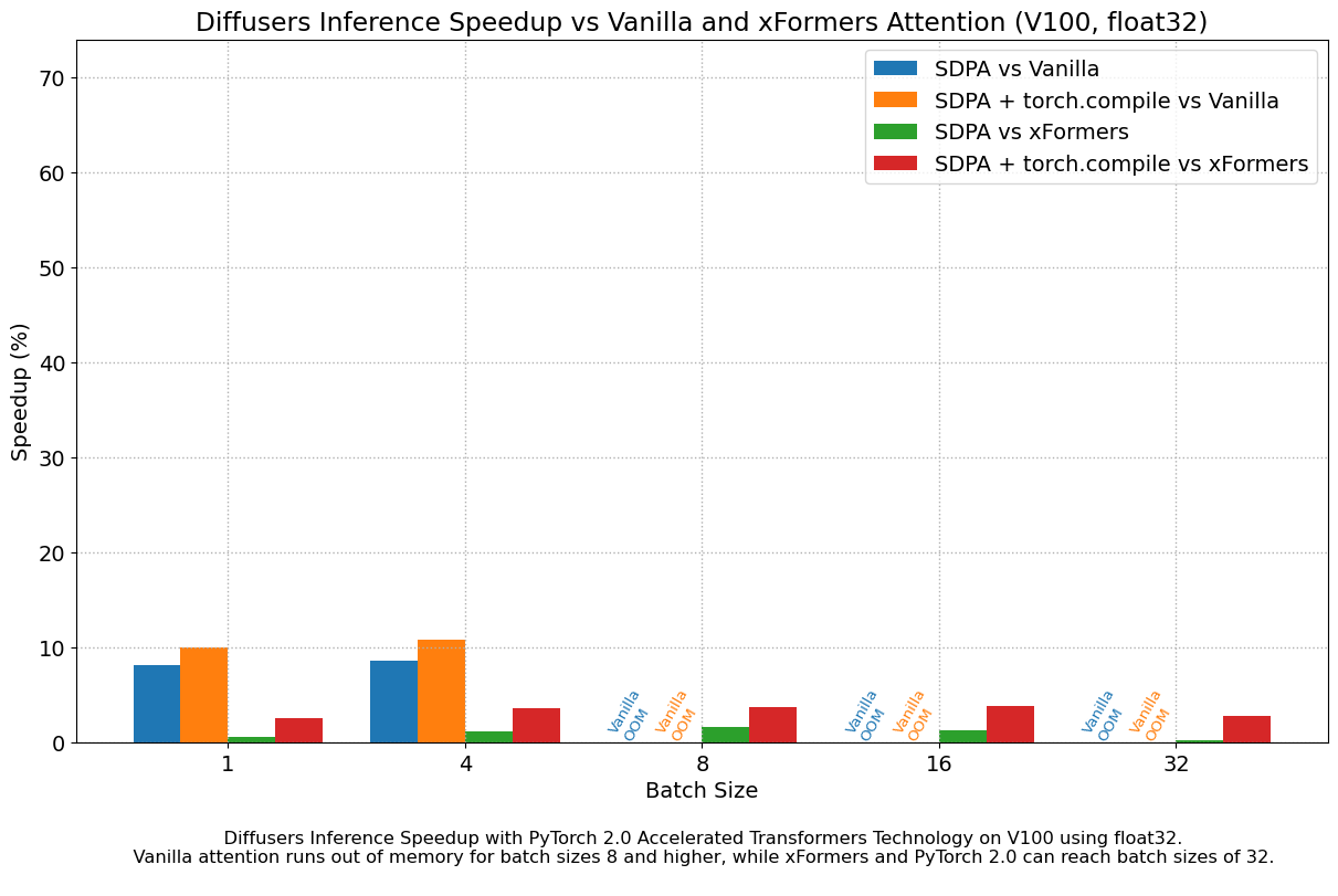
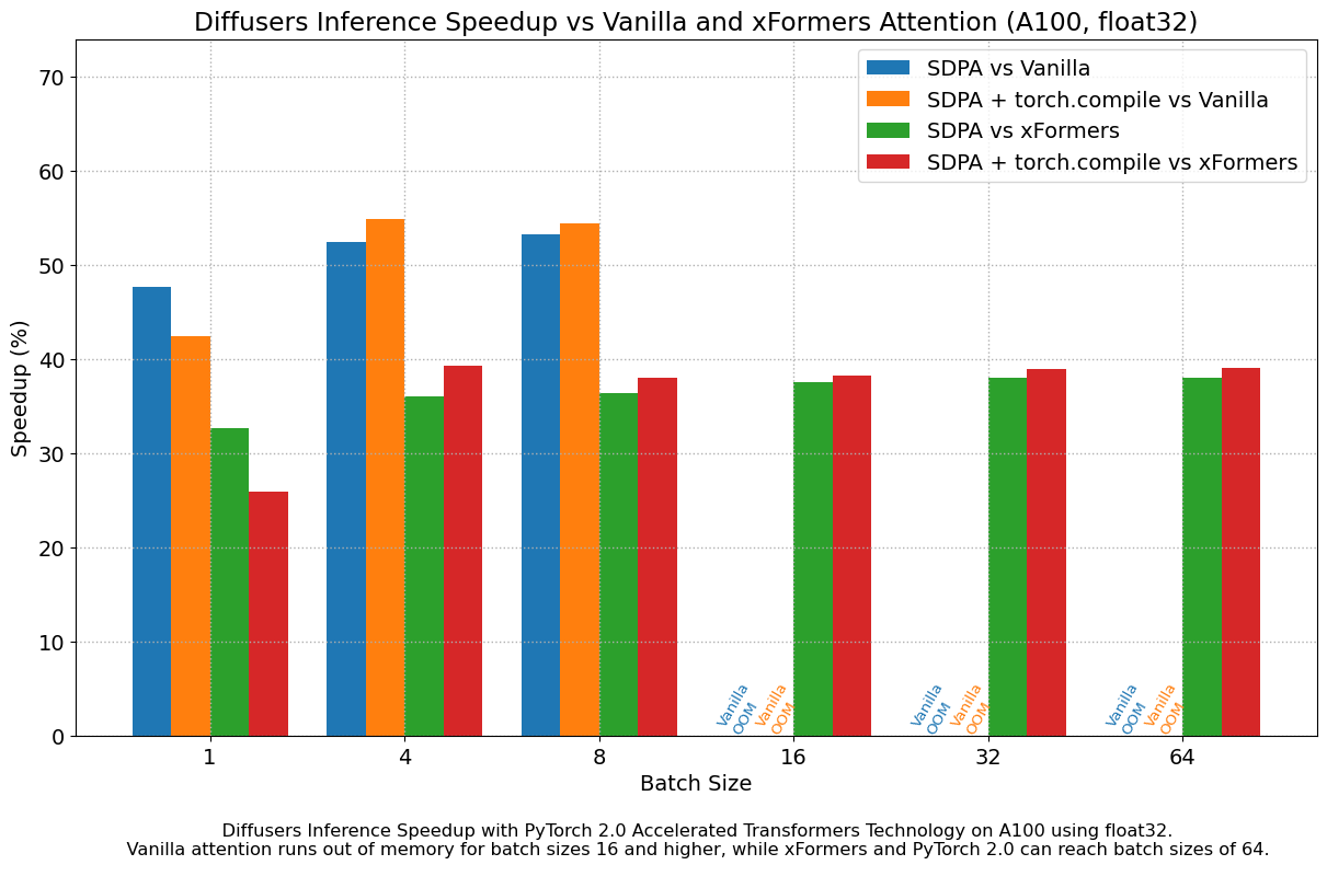
아마 a100 에서는 FlashAttention 을 사용할 수 있기때문에 더 빨라지는거 같고 비교군 중 diffusers 의 vanilla attention 은 제가 예시로 만든 것 처럼 단순한 attention 임을 알 수 있습니다. 이번 subsection에서 궁금한 것은 xformers와의 performance 비교 입니다. 먼저 아래처럼 간단하게 package를 설치해줍니다.

pip install -U xformers &&
python -m xformers.info

제대로 설치됐다면 아래처럼 볼 수 있습니다.

xFormers 0.0.17
memory_efficient_attention.cutlassF:               available
memory_efficient_attention.cutlassB:               available
memory_efficient_attention.flshattF:               available
memory_efficient_attention.flshattB:               available
memory_efficient_attention.smallkF:                available
memory_efficient_attention.smallkB:                available
memory_efficient_attention.tritonflashattF:        available
memory_efficient_attention.tritonflashattB:        available
swiglu.dual_gemm_silu:                             available
swiglu.gemm_fused_operand_sum:                     available
swiglu.fused.p.cpp:                                available
is_triton_available:                               True
is_functorch_available:                            False
pytorch.version:                                   2.0.0+cu117
pytorch.cuda:                                      available
gpu.compute_capability:                            7.0
gpu.name:                                          Tesla V100-SXM2-32GB
build.info:                                        available
build.cuda_version:                                1108
build.python_version:                              3.8.16
build.torch_version:                               2.0.0+cu118
build.env.TORCH_CUDA_ARCH_LIST:                    5.0+PTX 6.0 6.1 7.0 7.5 8.0 8.6                                                                   
build.env.XFORMERS_BUILD_TYPE:                     Release
build.env.XFORMERS_ENABLE_DEBUG_ASSERTIONS:        None
build.env.NVCC_FLAGS:                              None
build.env.XFORMERS_PACKAGE_FROM:                   wheel-v0.0.17
source.privacy:                                    open source

xformers docs 를 보면 Memory-efficient attention 구현체의 사용법을 볼 수 있습니다. 아래의 naive SDPA 와 대응되지만

scale = 1 / query.shape[-1] ** 0.5
query = query * scale
attn = query @ key.transpose(-2, -1)
if attn_bias is not None:
    attn = attn + attn_bias
attn = attn.softmax(-1)
attn = F.dropout(attn, p)
return attn @ value

memory 를 덜 먹는 연산을 해주는건데요,

import xformers.ops as xops

# Compute regular attention
y = xops.memory_efficient_attention(q, k, v)

# With a dropout of 0.2
y = xops.memory_efficient_attention(q, k, v, p=0.2)

# Causal attention
y = xops.memory_efficient_attention(
    q, k, v,
    attn_bias=xops.LowerTriangularMask()
)

출력값과 속도를 비교해봅시다.

import xformers.ops as xops
def forward_mem_efficient_xformers(q, k, v, bsz, n_head, d_k):
    out = xops.memory_efficient_attention(q, k, v)
    return out.contiguous().view(bsz, -1, n_head * d_k)

위 구현체는 torch SDPA 와 다르게 B, T, H, C shape 의 입력을 받습니다.

q = linear_q(x).view(bsz, -1, n_head, d_k).transpose(1, 2) # B, H, T, C
k = linear_k(x).view(bsz, -1, n_head, d_k).transpose(1, 2) # B, H, T, C
v = linear_v(x).view(bsz, -1, n_head, d_k).transpose(1, 2) # B, H, T, C

## for xformers
q_ = q.transpose(1,2) # B, H, T, C -> B, T, H, C
k_ = k.transpose(1,2) # B, H, T, C -> B, T, H, C
v_ = v.transpose(1,2) # B, H, T, C -> B, T, H, C

먼저 sequence length 100 에 대해서 비교해봅시다.

bsz = 4
n_head = 8
n_feat = 768
seq_len = 100

out = forward_attention(q, k, v, bsz, n_head, d_k)
out1 = linear_out(out)

out = forward_mem_efficient_xformers(q_, k_, v_, bsz, n_head, d_k)
out2 = linear_out(out)

print("all close : {}".format(torch.allclose(out1, out2, atol=1e-2, rtol=0)))
print("diff max : {}".format((out1-out2).abs().max()))
print("diff mean : {}".format((out1-out2).abs().mean()))

print(f"Naive SDPA implementation runs in {benchmark_torch_function_in_microseconds(forward_attention, q, k, v, bsz, n_head, d_k):.3f} microseconds")
print(f"The default torch builtin SDPA implementation runs in {benchmark_torch_function_in_microseconds(forward_efficient_sdpa, q, k, v, bsz, n_head, d_k):.3f} microseconds")
print(f"The default xops.memory_efficient_attention runs in {benchmark_torch_function_in_microseconds(forward_mem_efficient_xformers, q_, k_, v_, bsz, n_head, d_k):.3f} microseconds")

v100 에서 performance 는 다음과 같습니다.

all close : True
diff max : 2.682209014892578e-07
diff mean : 4.08217957215129e-08

Naive SDPA implementation runs in 170.225 microseconds
The default torch builtin SDPA implementation runs in 29.693 microseconds
The default xops.memory_efficient_attention runs in 201.639 microseconds

torch built-in sdpa 가 더 빠릅니다. 이번에는 length 를 512로 늘려봅시다.

all close : True
diff max : 5.066394805908203e-07
diff mean : 7.635312471165889e-08

Naive SDPA implementation runs in 597.752 microseconds
The default torch builtin SDPA implementation runs in 403.114 microseconds
The default xops.memory_efficient_attention runs in 404.556 microseconds

길이가 길어질수록 서로 비슷해지는걸 볼 수 있습니다. sequence length 별로 plot해보겠습니다.

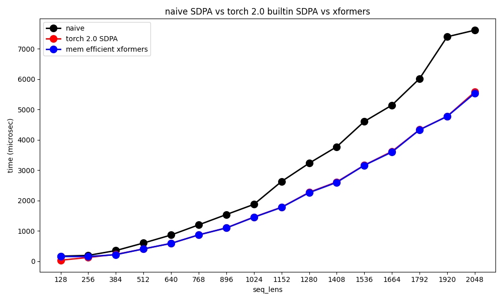sdpa_comparison_time_v100 Fig. v100 benchmarking

xformers 가 torch에 계속 업데이트되고 있어서 그런지 실제 속도차이는 거의 나지 않습니다. 그러면 다른 hardward 로 해볼까요?

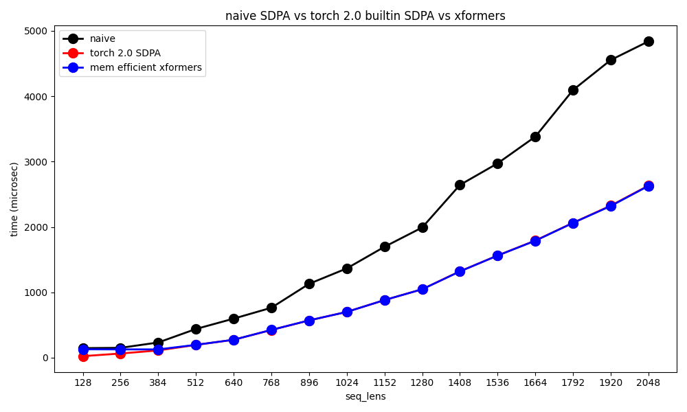sdpa_comparison_time_a100 Fig. A100 benchmarking

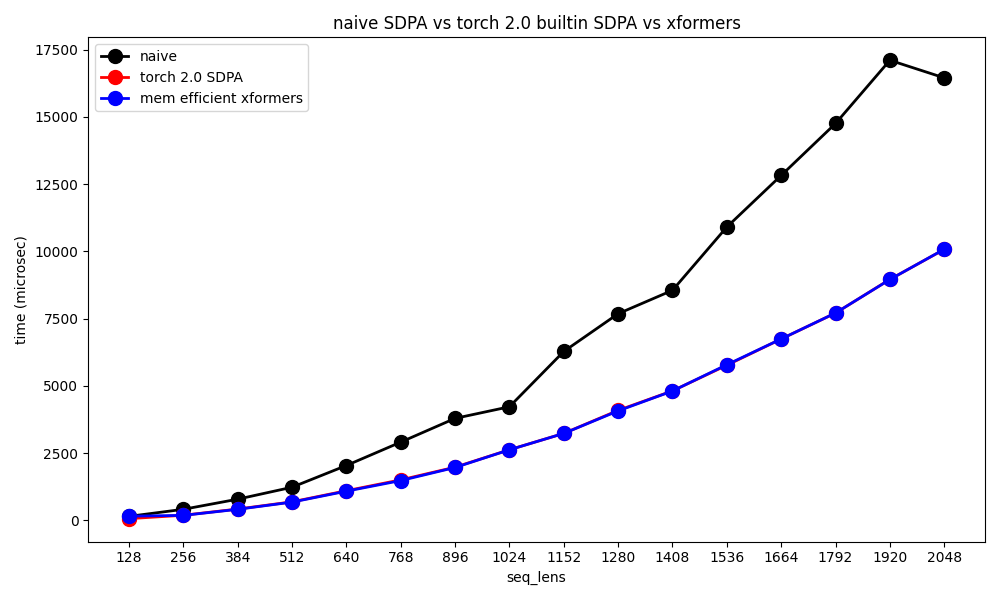sdpa_comparison_time_p40 Fig. p40 benchmarking

역시 A100 은 굉장히 비싸고 좋은 gpu 임을 알 수 있다.

How to Inject Relative Positional Information in xformers

Attention Bias (ALiBi or TFXL RPE)

NotImplementedError: No operator found for `memory_efficient_attention_forward` with inputs:                                                                                  
     query       : shape=(4, 100, 8, 96) (torch.float16)
     key         : shape=(4, 100, 8, 96) (torch.float16)
     value       : shape=(4, 100, 8, 96) (torch.float16)
     attn_bias   : <class 'torch.Tensor'>
     p           : 0.0
`flshattF` is not supported because:
    attn_bias type is <class 'torch.Tensor'>
    requires a GPU with compute capability > 7.5
`tritonflashattF` is not supported because:
    attn_bias type is <class 'torch.Tensor'>
    requires A100 GPU
`cutlassF` is not supported because:
    attn_bias.stride(-2) % 8 != 0 (attn_bias.stride() = (10000, 100, 1))
    HINT: To use an `attn_bias` with a sequence length that is not a multiple of 8, you need to ensure memory is aligned by slicing a bigger tensor. Example: use `attn_bias =
torch.zeros([1, 1, 5, 8])[:,:,:,:5]` instead of `torch.zeros([1, 1, 5, 5])`
`smallkF` is not supported because:
    dtype=torch.float16 (supported: {torch.float32})
    max(query.shape[-1] != value.shape[-1]) > 32
    bias with non-zero stride not supported
    unsupported embed per head: 96

update: 24. 02. 09: now flash attention support efficient ALiBi (contribution from research engineer of kakaobrain)

RoPE

그다음 Rotary Positional Encoding (RoPE)을 사용하는 방법이다.

Lightning-AI/lit-llama/lit_llama/model.py

Benchmarks on Real-World Model and Dataset

이번에는 실제 training, inference에 쓰이는 model을 기준으로 비교해보자. Training, inferece시 어디가 bottleneck인지 확인하는 tool에는 Nvidia의 Nsight, Pytorch Profiler같은 것들이 있을 수 있는데, Nsight가 좀 더 사용하기 귀찮기 때문에 torch profiler를 써보도록 하겠다. (사실 torch profiler도 기능이 너무 많고 cuda operator들이 async하게 호출되기 때문에 구체적으로 보기는 쉽지 않다)

RoBERTa Large

먼저 RoBERTa Large 모델에 대해서 xformers나 torch built-in sdpa 를 쓰면 실제로 얼마나 개선이 있을지에 대해 알아보자. RoBERTa Lrage는 Transformer Block 이 24개나 쌓여있어 355M 정도 parameter size 를 갖는 모델로 MHA과 FFN이 주된 computational bottleneck 이다.

num. shared model params: 355,411,033 (num. trained: 355,411,033)
RobertaHubInterface(
  (model): RobertaModel(
    (encoder): RobertaEncoder(
      (sentence_encoder): TransformerEncoder(
        (dropout_module): FairseqDropout()
        (embed_tokens): Embedding(50265, 1024, padding_idx=1)
        (embed_positions): LearnedPositionalEmbedding(514, 1024, padding_idx=1)
        (layernorm_embedding): LayerNorm((1024,), eps=1e-05, elementwise_affine=True)
        (layers): ModuleList(
          (0-23): 24 x TransformerEncoderLayerBase(
            (self_attn): MultiheadAttention(
              (dropout_module): FairseqDropout()
              (k_proj): Linear(in_features=1024, out_features=1024, bias=True)
              (v_proj): Linear(in_features=1024, out_features=1024, bias=True)
              (q_proj): Linear(in_features=1024, out_features=1024, bias=True)
              (out_proj): Linear(in_features=1024, out_features=1024, bias=True)
            )
            (self_attn_layer_norm): LayerNorm((1024,), eps=1e-05, elementwise_affine=True)
            (dropout_module): FairseqDropout()
            (activation_dropout_module): FairseqDropout()
            (fc1): Linear(in_features=1024, out_features=4096, bias=True)
            (fc2): Linear(in_features=4096, out_features=1024, bias=True)
            (final_layer_norm): LayerNorm((1024,), eps=1e-05, elementwise_affine=True)
          )
        )
      )
      (lm_head): RobertaLMHead(
        (dense): Linear(in_features=1024, out_features=1024, bias=True)
        (layer_norm): LayerNorm((1024,), eps=1e-05, elementwise_affine=True)
      )
    )
    (classification_heads): ModuleDict()
  )
)

먼저 xformers나 torch built-in sdpa가 아닌 구현체에 대해서 batch size 512, sequence length 512 인 dummy tensor 를 만들어 forwarding 해보자. wait step 1, warmup step 2번을 가지고 나머지 2 step을 기록한다. 지금은 inference bottleneck 에 관심이 있기 때문에 torch.no_grad() 환경에서 profiling 을 진행했다.

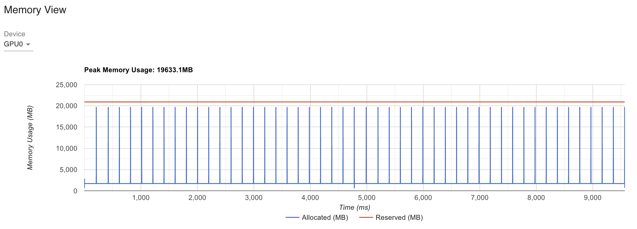roberta_large_512_512_naive Fig. Inference Performance of Naive SDPA applied Roberta for same input

위의 figure 를 보면 model이 forward를 하면서 갖는 Peak Memory가 19,633.1MB 임을 알 수 있는데, 이는 Transformer 한 블럭을 forwarding 할 때 memory이다 (RoBERTa 의 경우 MHA -> Norm -> FFN -> Norm 을 24번 반복). 그리고 시간도 2 step에 대해서 9,000ms가 넘게 걸렸다. 이번에는 torch built-in sdpa 와 memory efficient xformer 커널을 써보자.

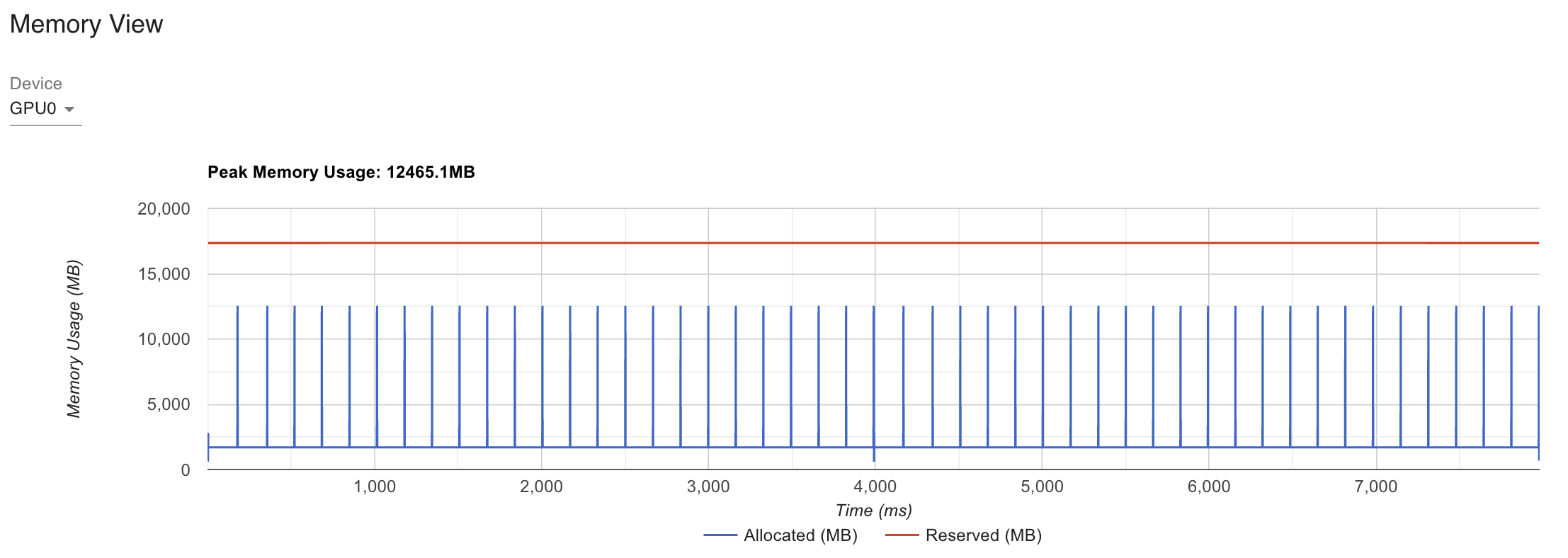roberta_large_512_512_torch_sdpa Fig. Inference Performance of Torch SDPA applied Roberta for same input

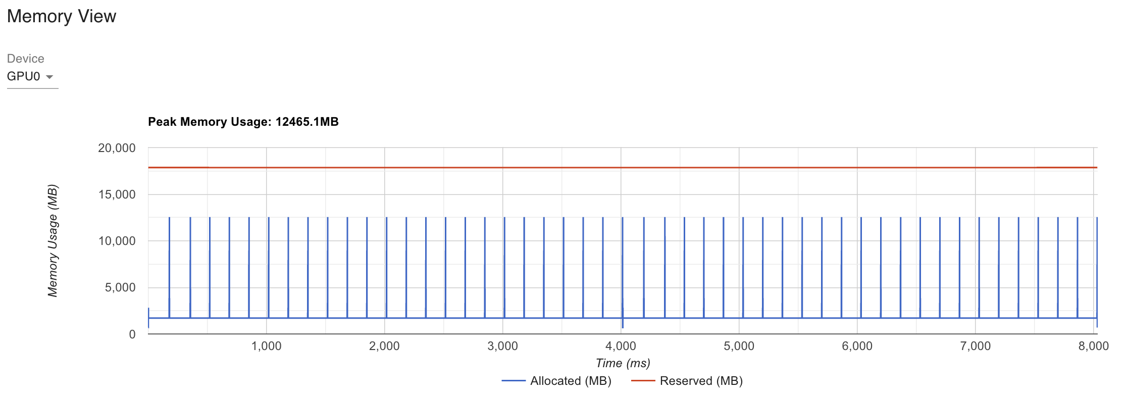roberta_large_512_512_xformers Fig. Inference Performance of xformers SDPA applied Roberta for same input

GPU Peak Memory 가 7000가까이 줄어든 걸 볼 수 있고 latency 도 10% 넘게 개선된 것을 알 수 있다. 여기서 torch profiler나 nvidia-smi를 쓸 때 알아둬야 할 점은 reservation이 torch가 gpu memory가 이정도 들 것으로 예상하고 예약을 잡아둔 것이라 실제 inference에 쓰인 memory를 의미하지는 않는다는 것이다. 그럼에도 불구하고 확실한 memory footprint improvement가 있었음을 확인할 수 있다.

Notes