CrossEntropyLoss vs NLL (feat. REINFORCE)
01 May 2022< 목차 >
How to optimize objective funcion in DL?
Classification task를 풀기 위해서는 하면 Cross Entropy (CE) loss를 objective function으로 쓰게 된다. Model이 실제로 추론한 값, \(\hat{y}\)와 정답에 해당하는 gold label, \(y\)에 대해서 CE Loss 를 계산하기 위한 pytorch implementation은 아래와 같다.
import torch
import torch.nn as nn
import torch.nn.functional as F

input = torch.randn(2, 2, requires_grad=True)
target = torch.tensor([1, 0])
bce_loss = F.cross_entropy(input, target)
Binary classification을 하기 위해 toy logit을 만들고 loss를 계산하면 아래와 같은 결과를 확인할 수 있다.
>>> input
tensor([[ 0.6790,  0.1083],
        [-0.2791,  0.0378]], requires_grad=True)
>>> target
tensor([1, 0])
>>> bce_loss
tensor(0.9414, grad_fn=<NllLossBackward0>)
BCE를 사용해서 조금 설명을 해 보도록 하겠다. 이를 torch docs에 있는 수식으로 표현하면 아래와 같다. (Docs > torch.nn > BCELoss와 Docs > torch.nn > CrossEntropyLoss를 참고)
\[\ell(x, y)=L=\{l_{1}, \ldots, l_{N}\}^{\top}, \quad l_{n}=-w_{n}\left[y_{n} \cdot \log x_{n}+\left(1-y_{n}\right) \cdot \log \left(1-x_{n}\right)\right]\] \[\ell(x, y)= \begin{cases}\operatorname{mean}(L), & \text { if reduction }=\text { 'mean' } \\ \operatorname{sum}(L), & \text { if reduction }=\text { 'sum' }\end{cases}\]여기서 \(w_n\), loss weight는 일반적으로 data에 불균형이 있지 않는 이상 사용하지 않는다. BCE는 CE의 special case이기 때문에 CE Loss 도 비슷하게 계산을 할 수 있다. (그냥 같은 것)
\[\ell(x, y)=L=\{l_{1}, \ldots, l_{N}\}^{\top}, \quad l_{n}=-w_{y_{n}} \log \frac{\exp (x_{n, y_{n}})}{\sum_{c=1}^{C} \exp (x_{n, c})} \cdot 1 \{ y_{n} \neq \text{ignore index} \}\] \[\ell(x, y)= \begin{cases}\sum_{n=1}^{N} \frac{1}{\sum_{n=1}^{N} w_{y_{n}} \cdot 1\left\{y_{n} \neq \text { ignore index }\right\}} l_{n}, & \text { if reduction = 'mean' } \\ \sum_{n=1}^{N} l_{n}, & \text { if reduction }=\text { 'sum' }\end{cases}\]CE loss는 본래 내가 가지고있는 dataset의 target distribution을 categorical distribution 정하는 것이며, 확률은 합이 1이 되어야 하므로 softmax function으로 normalize 해 줬음을 알 수 있다. BCE는 bernoulli distribution을 modeling하는데 category가 2개뿐이었으므로 sigmoid function을 사용했다는 점에서 약간 차이가 있을 뿐이다. CE loss 또한 pytorch framework을 쓰면 아래와 같이 간단하게 계산해볼 수 있다.
input = torch.randn(4, 5, requires_grad=True)
target = torch.tensor([1, 0, 4, 2])
ce_loss = F.cross_entropy(input, target)
>>> input; target; ce_loss;
tensor([[-1.1116,  1.3008, -1.7689, -0.6705,  1.3516],
        [ 2.1148, -1.0967, -0.7057,  0.1985,  0.1819],
        [ 0.1373, -0.1615,  0.9620,  0.3299, -0.6667],
        [-1.4306, -1.1321,  0.1686, -1.4781,  0.5021]], requires_grad=True)
tensor([1, 0, 4, 2])
tensor(1.2090, grad_fn=<NllLossBackward0>)
CE vs (NLL + Log Softmax)
이제 CE loss를 numpy스럽게 직접 구현해보려고 한다. CE objective는 사실 softmax function으로 normalize한 logit tensor에 negative log를 취하는 것과 동치인데, numerical stability를 위해서 실제로는 log softmax와 NLL method의 조합을 사용해서 계산한다. 실제 torch의 softmax class를 보면 softmax를 쓰는 것 보다 log softmax를 쓰는 것이 더 빠르고 안정적이라고 하며 당연히 NLL과 결합되는 입장에서는 정확하게 동일한 연산이므로 문제가 없다고 한다.
log_softmax = F.log_softmax(input, dim=-1)
nll_loss = F.nll_loss(log_softmax, target)
assert torch.allclose(ce_loss, nll_loss), f"they are different {ce_loss} vs {nll_loss}"
여기서 torch.allclose란 두 tensor가 같은지 확인하는 pytorch 내장함수인데, 전혀 문제가 없음을 확인할 수 있다. 이제 CE loss 구현을 한꺼풀 더 벗겨보도록 하자. NLL method는 log softmax와 결합되지만 numerical stability를 무시하고 ‘softmax -> 정답 lable에 해당하는 logit을 lookup -> log -> 음수’를 취하는 계산 과정을 직접 구현해보자.
# Normalize and Look-up
softmax = F.softmax(input, dim=-1)
one_hot_target = F.one_hot(target)
look_up_softmax_probs = torch.gather(softmax, 1, target.unsqueeze(-1))
# Negative Log
log_probs = torch.log(look_up_softmax_probs)
loss = torch.mean(-log_probs)
assert torch.allclose(ce_loss, loss), f"they are different {ce_loss} vs {loss}"
위 세 가지 구현이 전부 동일한 것을 확인할 수 있었다.
REINFORCE
그런데 이걸 왜 까봤느냐? 사실 본 post의 주제는 REINFORCE를 구현하는 것이다. 이 밖에도 InfoNCE Loss등 다른 pytorch 에 존재하지 않는 objective function을 구현하기 위해서는 log_softmax와 NLL function을 자유자재로 쓸 줄 알아야 한다.
CE loss로 Supervised Learning (SL)을 하는 것은 REINFORCE의 special case라고 할 수 있다. 예를 들어 model이 5개 class에 대한 값을 return한다고 할 때, 해당 input의 정답이 4번째 class라면 4번째 logit만 lookup해서 -log를 취해 sample 하나에 대한 loss를 계산한다. 이를 모든 batch에 대해 병렬 처리해서 계산하면 모든 batch의 loss를 구하는 것이 된다.
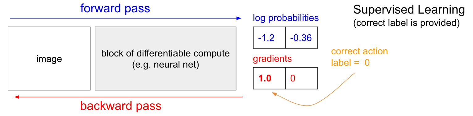 Fig. sL은 reward가 1인 REINFORCE algorithm의 special case라고 할 수 있다. Source From Andrej Karpathy’s Blog
REINFORCE는 Reinforcement Learning (RL)에서 policy network를 directly optimizate하는 method로, agent가 어떤 action을 했을 때 이것이 정답인지?에 대한 정보가 따로 존재하지 않는다. 그러면 어떻게 ‘이 행동이 좋았는가?’를 평가할 수 있을까. 예를 들어 시간이 흐름에 따라 network가 선택한 action이 아래와 같았다고 치자.
state (t=0) -> action 1
state (t=1) -> action 0
state (t=2) -> action 1
state (t=3) -> action 2
state (t=4) -> action 4
5번 action을 하면 하나의 episode가 끝난것이다.
그러면 각 action에 대해 environment가 이 action이 얼마나 좋았는지?를 나타내는 scalar reward를 알려준다.
자세한 사항은 이 post를 참고하면 되겠으나 직므 중요한 것은 RL에서는 정답이 따로 없고 내 action에 대한 scalar reward가 주어질 뿐이라는 것이다.
이런 경우 loss를 - (4번째 class의 log_prob * Reward)같은 방식으로 계산하게 된다.
즉 언제나 label이 주어져있고, 어떤 상황에서 그 label에 해당하는 logit을 lookup해 -log를 취하는 것과 다르게,
agent의 action에 -log를 취하고 reward만큼을 곱하는 이른 바 weighted CE loss를 구현해야 하는 것이다.
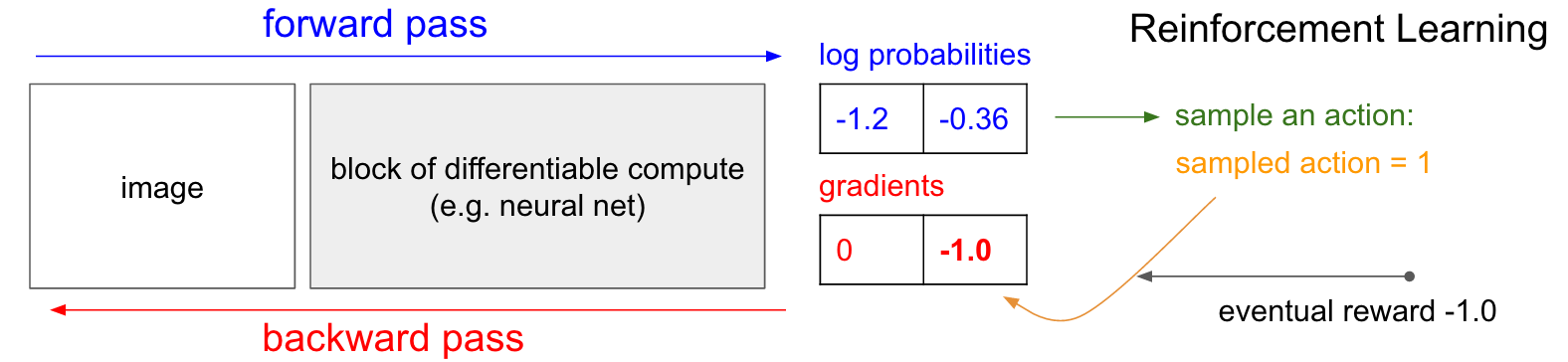 Fig. RL vs SL. Source From Andrej Karpathy’s Blog
REINFORCE의 loss는 아래처럼 구현할 수 있는데, logit에 log_softmax를 취해 얻은 log probability값에 reward를 곱하고 모든 batch, instance에서 계산된 값을 sum해서 backward를 취하면 gradient를 구할 수 잇게 된다.
    R = 0
    policy_loss = []
    returns = []
    for r in policy.rewards[::-1]:
        R = r + args.gamma * R
        returns.insert(0, R)
    returns = torch.tensor(returns)
    returns = (returns - returns.mean()) / (returns.std() + eps)
    for log_prob, R in zip(policy.saved_log_probs, returns):
        policy_loss.append(-log_prob * R)
    optimizer.zero_grad()
    policy_loss = torch.cat(policy_loss).sum()
    policy_loss.backward()
    optimizer.step()