(WIP) Dropout and Bayesian Deep Learning

< 목차 >

Overview
Training Neural Network (NN) with Dropout
Bayesian Neural Network (BNN)
- What's Wrong with BNN ?
Dropout as a Bayesian Approximation
- Gaussian Process (GP)
- Interperet Dropout as a Bayesian Approximation of GP
References

Overview

이 post는 Dropout과 Bayesian Approach 의 관계에 대한 내용을 담고 있다.

Dropout은 ML model이 training dataset에 과적합 (overfitting) 하는 것을 방지하는 정규화 (regularization) technique이다. 이는 학습 중 Neural Network (NN)의 일부 node를 확률적으로 on/off 하는 것으로 (2개의 class이므로 bernoulli distribution을 사용), dropout을 사용해 학습된 model이 generalize를 잘 하는 것은 ensemble관점에서 해석되는 경우가 많다.

Bayesian Deep Learning은 말 그대로 bayesian approach를 사용해 NN의 training, inference를 하는 것으로, ML model을 학습하는 것이 일반적으로 주어진 dataset, model parameter, objective (target distribution)이 있을 때 objective 를 가장 잘 만족시키는 parameter 하나를 찾는 point estimation을 하는 것에 불과할 때, bayesian approahc는 주어진 setting에서의 parameter의 distribution을 계산한 뒤 모든 parameter를 활용해 infernce한다. 다시 말해서 가능한 모든 parameter가 출력하는 각각의 distribution을 각 paramter의 확률로 weighted sum 하는 (사실상 integral) 것이다. 이럴 경우 연산이 많이 들지만 test time에 어떤 data에 대해 얼마나 model이 inference output을 낼 때 확신이 없는지 (uncertainty)와 같은 정보를 알 수있게 된다.

이 둘은 관련이 없어 보이지만 관련이 있다. 결론부터 말하자면 이 복잡하고 연산이 많이 드는 BNN은 사실 dropout 을 걸어 model training을 하는 것과 다름이 없고, 우리가 dropout을 걸어 maximum likelihood인 parameter를 찾는 것은 parameter의 distribution을 알려주지는 못해 input data에 대한 model의 uncertainty를 바로 얻을 순 없지만, dropout을 사용해 비슷한 효과를 낼 수 있다는 것이다. 이 모든 내용은 이 분야의 대가인 Yarin Gal의 학위 논문 (thesis), Uncertainty in Deep Learning에 자세하게 기술되어 있다. 본 post의 목적은 이를 잘 설명하는 것 이다.

We show that the use of dropout (and its variants) in NNs 
can be interpreted as a Bayesian approximation of a well known probabilistic model: 
the Gaussian process (GP) (Rasmussen & Williams, 2006). 

Training Neural Network (NN) with Dropout

먼저 dropout에 대해서 간단히 알아보자. 원래 idea는 bishop의 Training with Noise is Equivalent to Tikhonov Regularization라는 paper에서 제안되었다고 한다. 후에 비슷한 idea가 NN에 적용되면서 우리가 아는 paper, A Simple Way to Prevent Neural Networks from Overfitting가 제안된 것으로 보인다. Dropout은 말 그대로 학습 중 node를 일부 drop 시켜서 forwarding하고 loss를 계산하고 parameter update를 하는 방식이다. 그런데 이 neuren을 drop시키는 행위는 bernoulli distribution에 따라 확률적으로 발생한다.

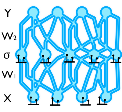do_net_gal Fig.

Dropout이 왜 작동하는지?에 대해서는 두 가지 설이 유력한데,

co-adaptation을 막아주기 때문에
model ensemble을 하는 효과를 내기 때문에

첫 번째는 예를 들어 어떤 고양이 image를 받아 이를 고양이로 분류하기 위해서 마지막 classifier layer의 경우 실제로는 물체의 눈, 코, 귀, 복슬복슬함 등 feature들을 종합적으로 보고 판단해야 하는데, dropout을 함으로써 눈, 귀는 못보게 한 뒤에 나머지 feature들만 보고 고양이임을 맞추게 함으로써 더 강력한 representation을 얻을 수 있게 하는것이다.

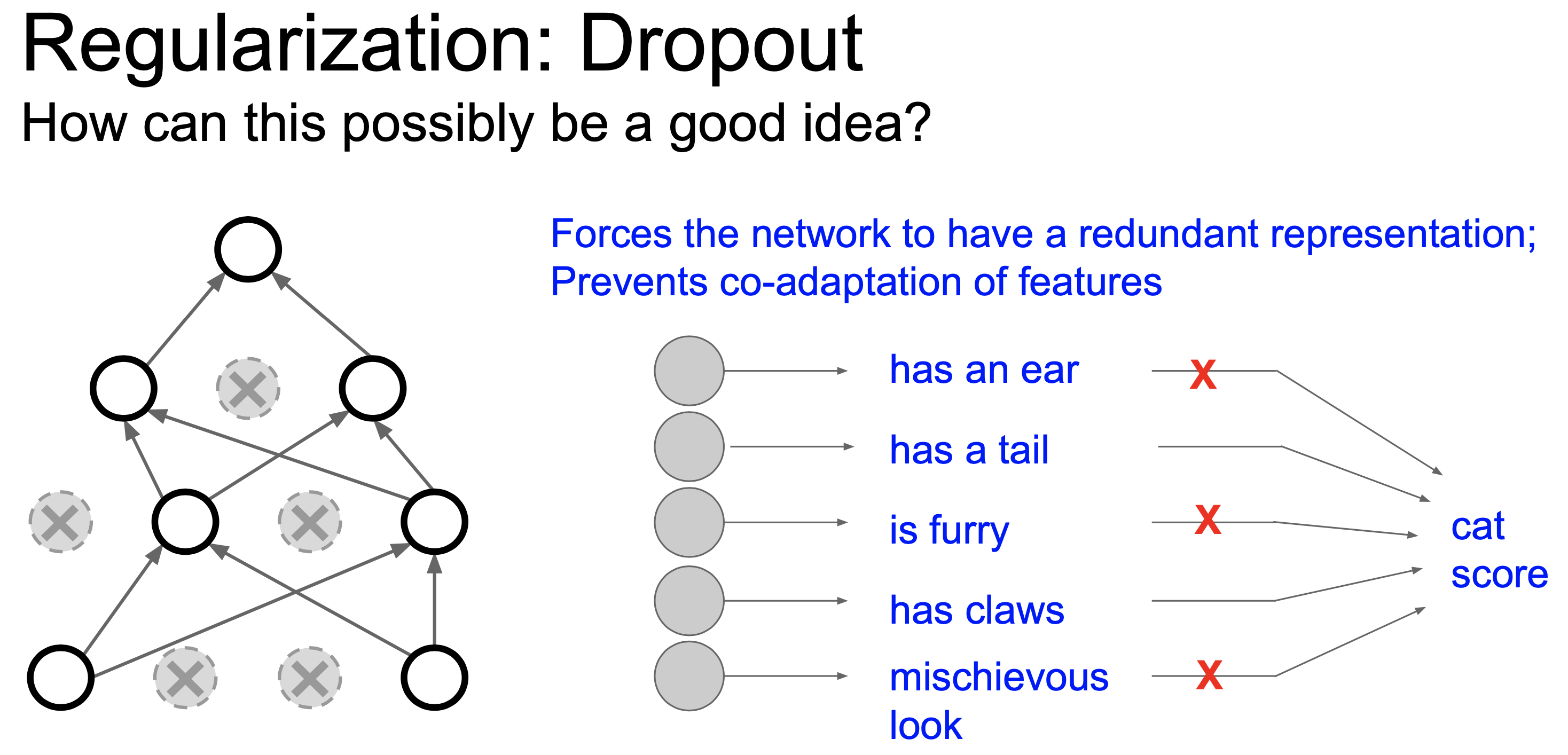dropout_explanation_fig2 Fig.

Co-adaptation는 공동 적응, 동조 쯤으로 해석되는데, dropout 없이 학습을 할 때는 모든 feature를 보고 고양이라고 판단하기 때문에 서로 다른 hidden unit이 높은 correlated behavior를 갖게 된다는 것이다. Paper에는 model이 학습되는 과정에서 (backprop) 어떤 neuron이 다른 neuron이 저지를 실수를 보완해주는 식으로 학습이 되면 강한 correlation이 생길 수 있다고 되어있다.

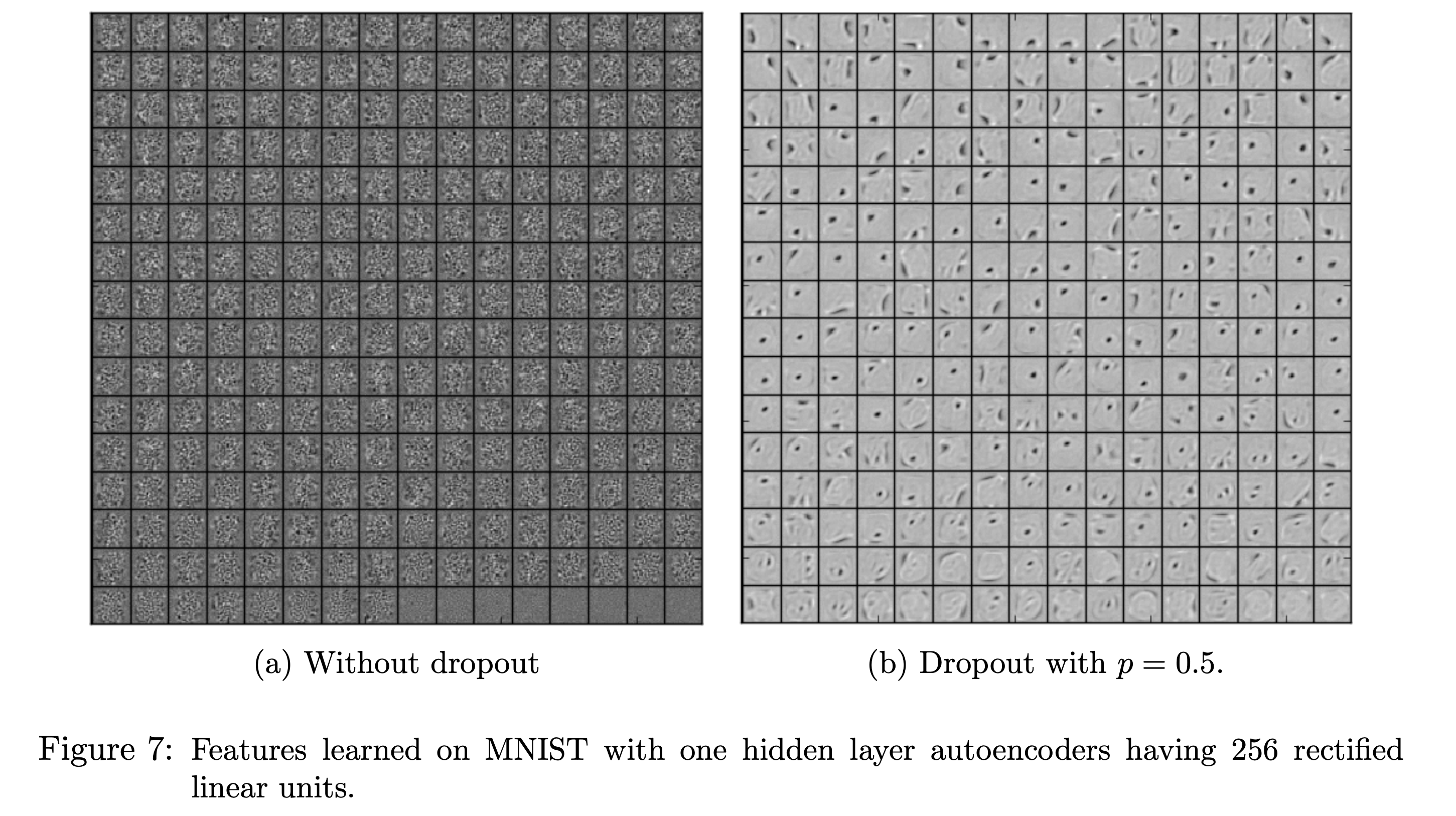dropout_paper_learned_feature Fig. Dropout이 적용된 Auto Encoder가 더 선명한 feature를 가지게 된다.

그 다음 model ensemble을 하는 효과를 낸다는 해석은 무작위로 dropout 처리된 서로 다른 model들은 서로 다른 model로 볼 수 있고 (왜냐면 parameter가 누락됐으니 다른 parameter set인 것), test time에 모든 node를 킨다는 것은 이 model들이 추론한 결과를 합친다 (ensemble)는 해석이 가능하기 때문이다.

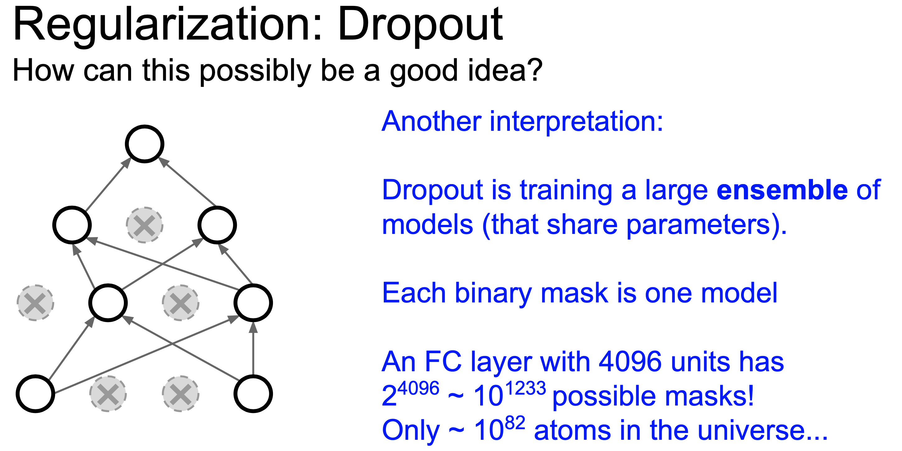dropout_explanation_fig3 Fig.

Dropout을 사용할 때 주의할 점은 training시에는 node가 drop된 형태로 forwarding되지만, inference시에는 그렇지 않다는 점이다. (그래서 ensemble이라고 얘기하는 사람이 있는 데 맞는 설명인 것 같다.)

그러므로 inference시에는 모든 node가 on/off될 가능성을 고려해서 expectation을 취한 값을 사용해야 하는데, 각 dropout rate은 bernoulli distribution을 따르기 때문에 실제로 dropout rate이 0.5라면 아래처럼 계산할 수 있다.

dropout_explanation_fig4 Fig.

그 결과 infernce시에 activation에 dropout probability만큼을 곱해주면 된다는 결론에 이른다. (실제로는 dropout시 prob을 오히려 나눠주는 것으로 구현되어있는데, 구현상의 편의를 위해 그런 것이고 결국 이 둘은 동치이며 후자를 inverted dropout 라고 부른다.)

Bayesian Neural Network (BNN)

What's Wrong with BNN ?

Dropout as a Bayesian Approximation

Gaussian Process (GP)

gp_net_gal Fig.

gpposterior0_cornell Fig.

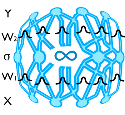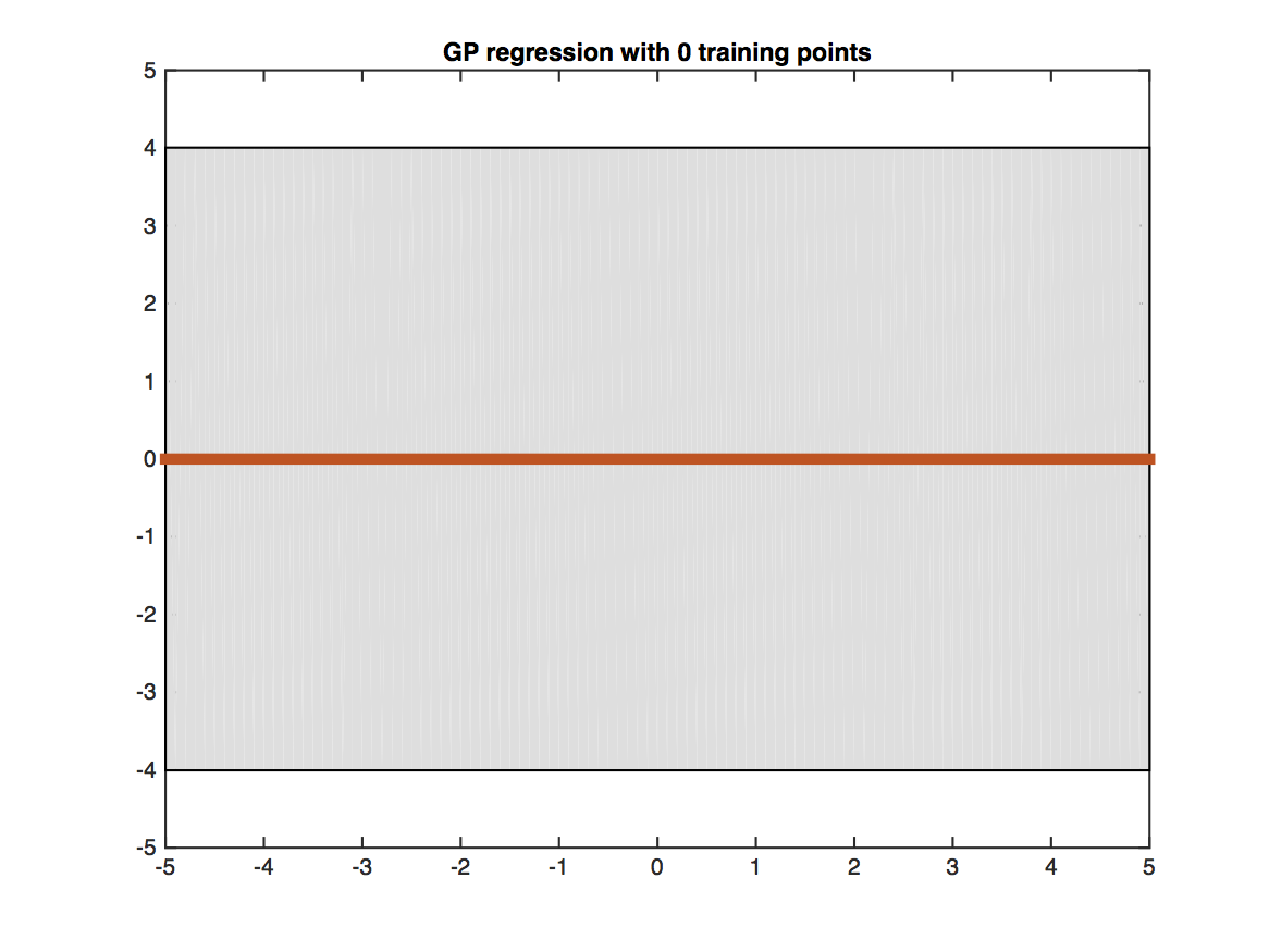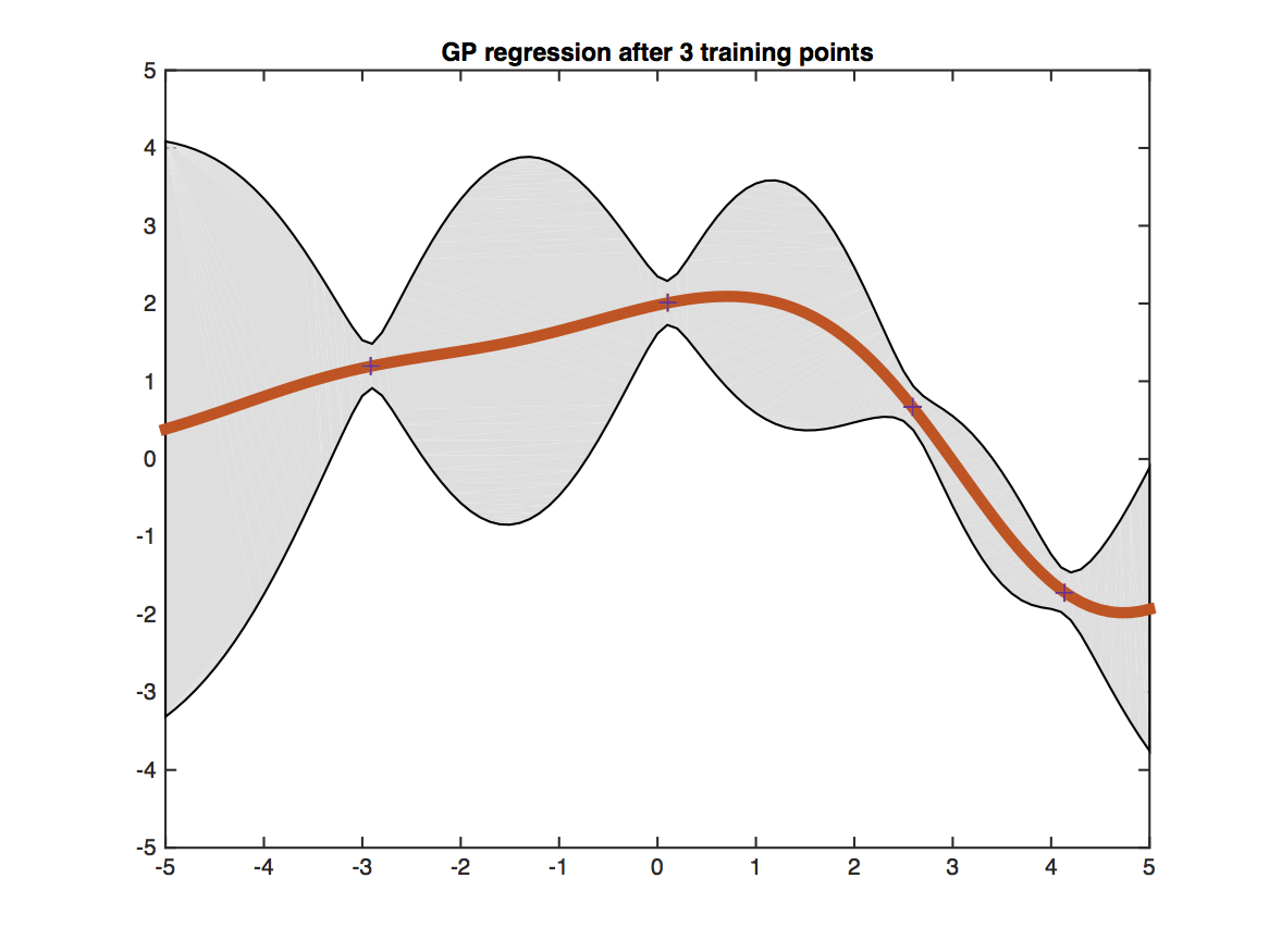gpposterior3_cornell Fig.

Interperet Dropout as a Bayesian Approximation of GP

\[\mathcal{L}_{\text {dropout }}:=\frac{1}{N} \sum_{i=1}^{N} E\left(\mathbf{y}_{i}, \widehat{\mathbf{y}}_{i}\right)+\lambda \sum_{i=1}^{L}\left(\left\|\mathbf{W}_{i}\right\|_{2}^{2}+\left\|\mathbf{b}_{i}\right\|_{2}^{2}\right)\] \[\mathbf{K}(\mathbf{x}, \mathbf{y})=\int p(\mathbf{w}) p(b) \sigma\left(\mathbf{w}^{T} \mathbf{x}+b\right) \sigma\left(\mathbf{w}^{T} \mathbf{y}+b\right) \mathrm{d} \mathbf{w} \mathrm{d} b\] \[\begin{gathered} p(\mathbf{y} \mid \mathbf{x}, \mathbf{X}, \mathbf{Y})=\int p(\mathbf{y} \mid \mathbf{x}, \boldsymbol{\omega}) p(\boldsymbol{\omega} \mid \mathbf{X}, \mathbf{Y}) \mathrm{d} \boldsymbol{\omega} \\ p(\mathbf{y} \mid \mathbf{x}, \boldsymbol{\omega})=\mathcal{N}\left(\mathbf{y} ; \widehat{\mathbf{y}}(\mathbf{x}, \boldsymbol{\omega}), \tau^{-1} \mathbf{I}_{D}\right)\widehat{\mathbf{y}}\left(\mathbf{x}, \boldsymbol{\omega}=\left\{\mathbf{W}_{1}, \ldots, \mathbf{W}_{L}\right\}\right) \\ =\sqrt{\frac{1}{K_{L}}} \mathbf{W}_{L} \sigma\left(\ldots \sqrt{\frac{1}{K_{1}}} \mathbf{W}_{2} \sigma\left(\mathbf{W}_{1} \mathbf{x}+\mathbf{m}_{1}\right) \ldots\right) \end{gathered}\] \[\begin{aligned} \mathbf{W}_{i} &=\mathbf{M}_{i} \cdot \operatorname{diag}\left(\left[\mathbf{z}_{i, j}\right]_{j=1}^{K_{i}}\right) \\ \mathbf{z}_{i, j} & \sim \operatorname{Bernoulli}\left(p_{i}\right) \text { for } i=1, \ldots, L, j=1, \ldots, K_{i-1} \end{aligned}\] \[-\int q(\boldsymbol{\omega}) \log p(\mathbf{Y} \mid \mathbf{X}, \boldsymbol{\omega}) \mathrm{d} \boldsymbol{\omega}+\mathbf{K L}(q(\boldsymbol{\omega}) \| p(\boldsymbol{\omega}))\]

Notes