(WIP) Distributional RL (Categorical DQN (C51), Quantile Regression DQN (QR-DQN) and so on)
04 Jan 2024< 목차 >
- Motivation
- Categorical DQN with 51 Category (C51)
- Quantile Regression DQN (QR-DQN)
- Implicit Quantile Network (IQN)
- References
Motivation
C51 (Categorical DQN with 51 Category) algorithm은 ICML 2017에 publish된 A Distributional Perspective on Reinforcement Learning에서 제안되었다. C51은 DQN과 같은 대표적인 value based method로 distribution RL이라는 category로 따로 분류된다.
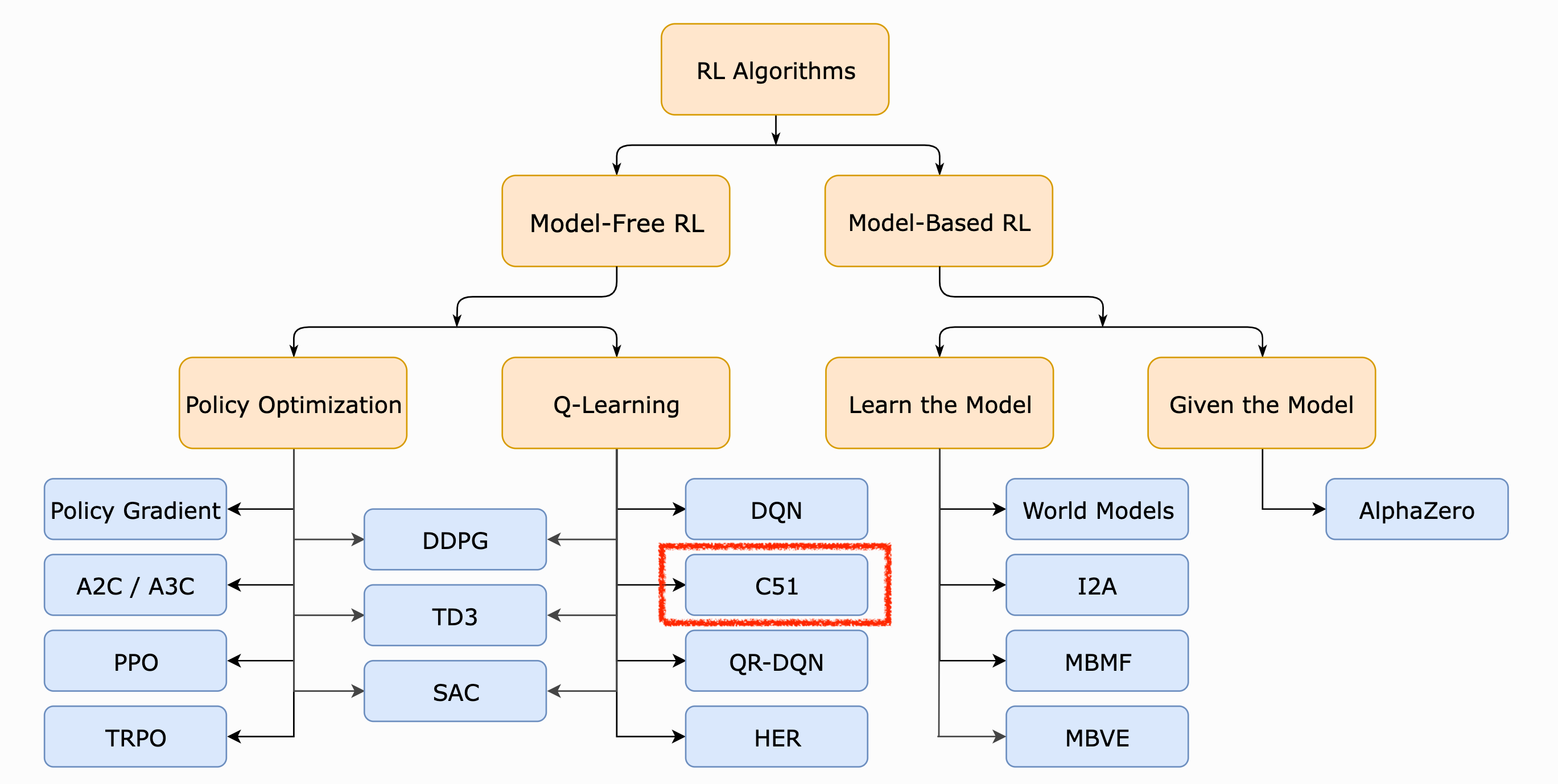 Fig.
Fig.
Distributional RL로 유명한 algorithm들은 크게 return의 dstribution을 modeling하느냐, 아니면 quantile function을 modeling하느냐로 나뉜고, C51은 return distribution을 modeling했다고 볼 수 있다.
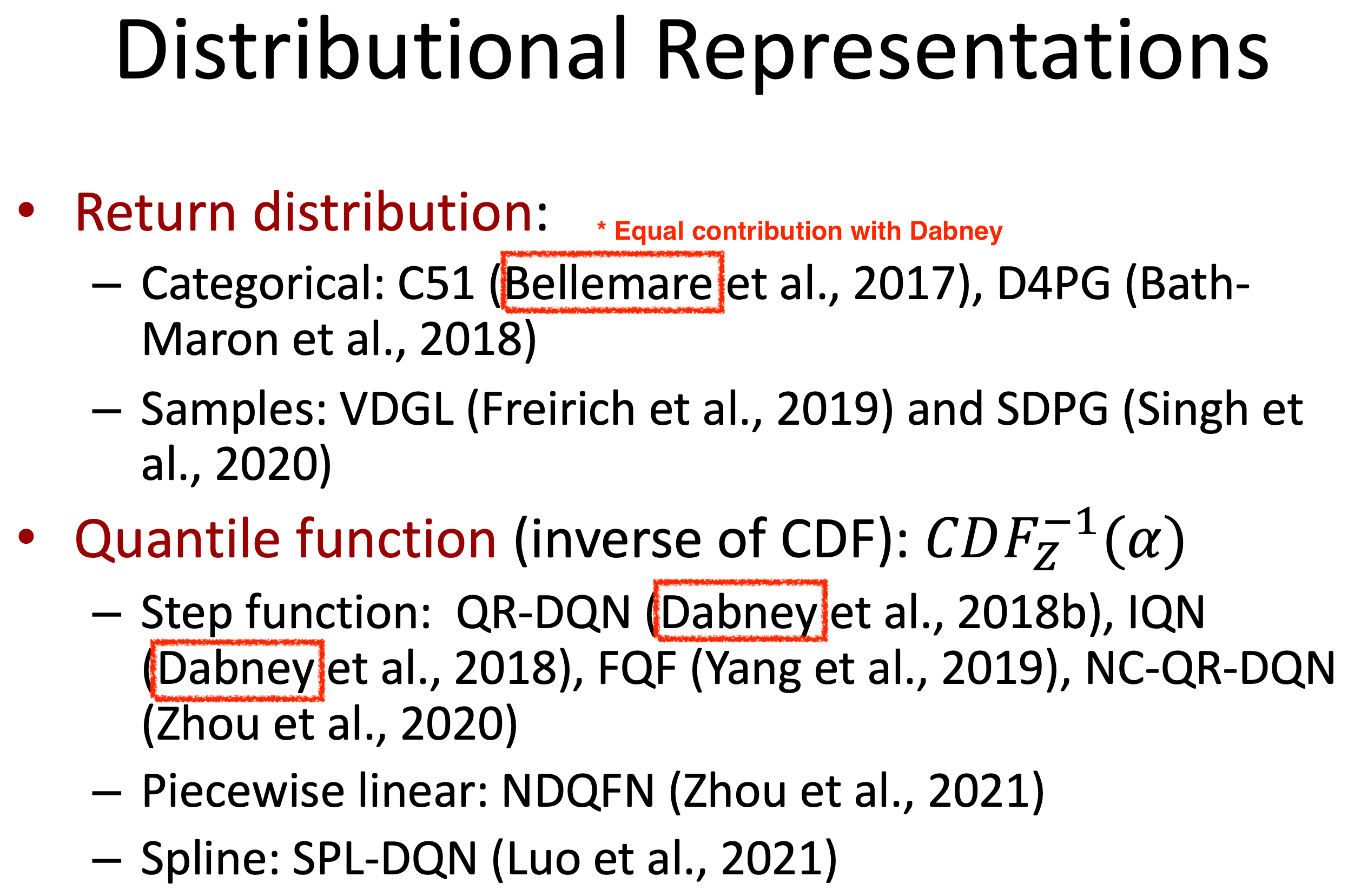 Fig. Will Dabney가 다 했다
왜 C51인가?
DQN은 어떤 state, \(s_t\)에서 어떤 action, \(a_t\)를 했을 때 그 action이 몇점짜리인지?를 학습한다.
즉 DQN algorithm이 regress하는 target은 \(s_t\)에서 \(a_t\)를 함으로써 발생가능한 trajectory들의 return의 expectation으로 scalar이다 (unimodal gaussian distribution).
즉 우리가 regress하는 target은 return distribution의 mean값인 것이다.
Distributional RL (DRL)은 return의 distribution 자체를 학습한다.
이 때 distribution이 51개 category를 갖는 categorical distribution이기 때문에 C51이라는 이름이 붙었다 (51은 magic number).
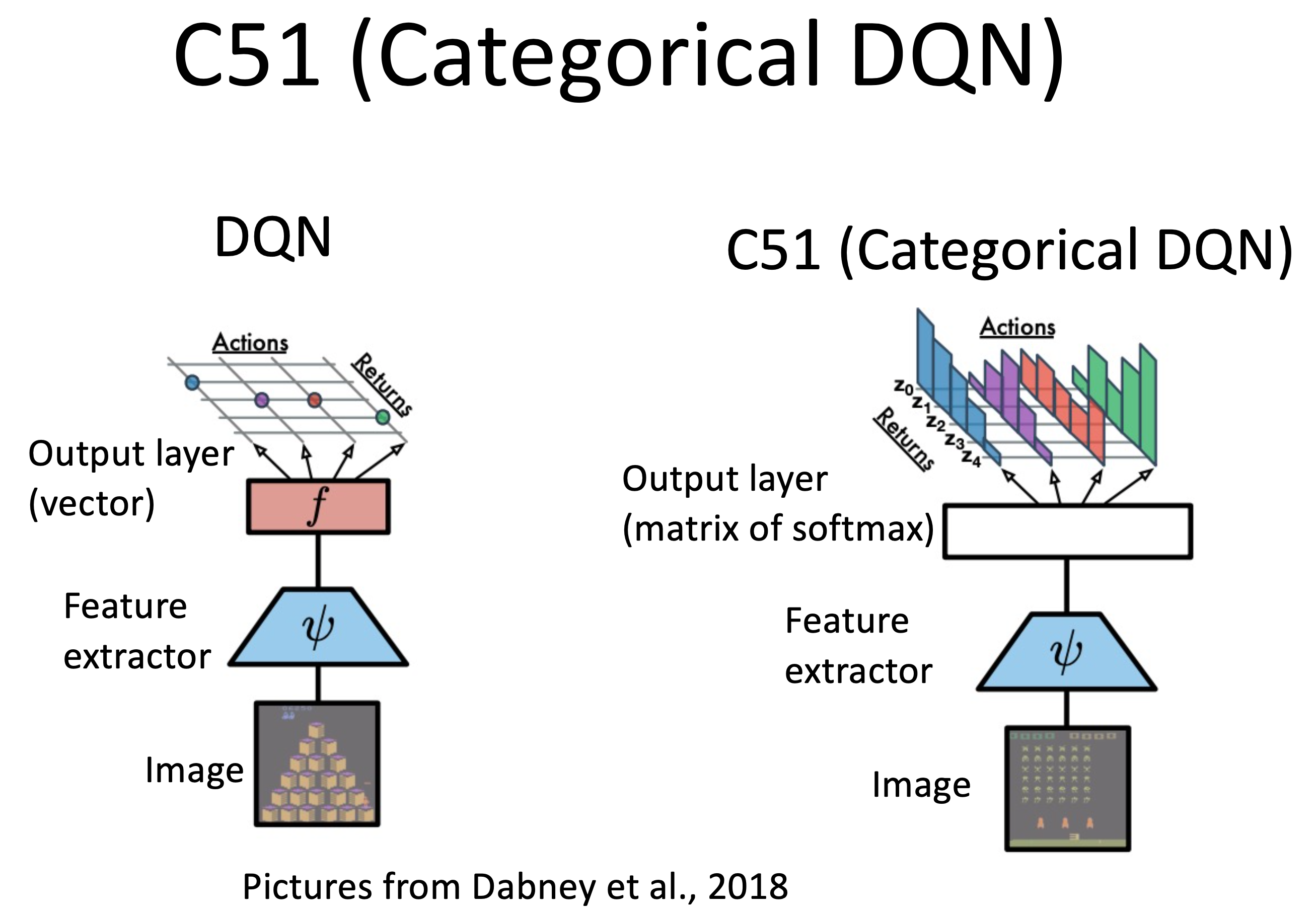 Fig.
Fig.
Why DRL?
왜 DRL을 해야할까? 아래의 예시를 생각해보자. Space invaders라는 game을 play하는 agent가 DRL로 학습된 경우이다. 당연히 inference시 NN, \(Q_{\phi}(s_t,a_t)\)가 return하는 것은 scalar가 아니라 distribution일 것이고, figure의 오른쪽에는 각 action을 했을 때 (action 별로 색이 다름) return의 distribution이 어떻게 되는지를 볼 수 있다.
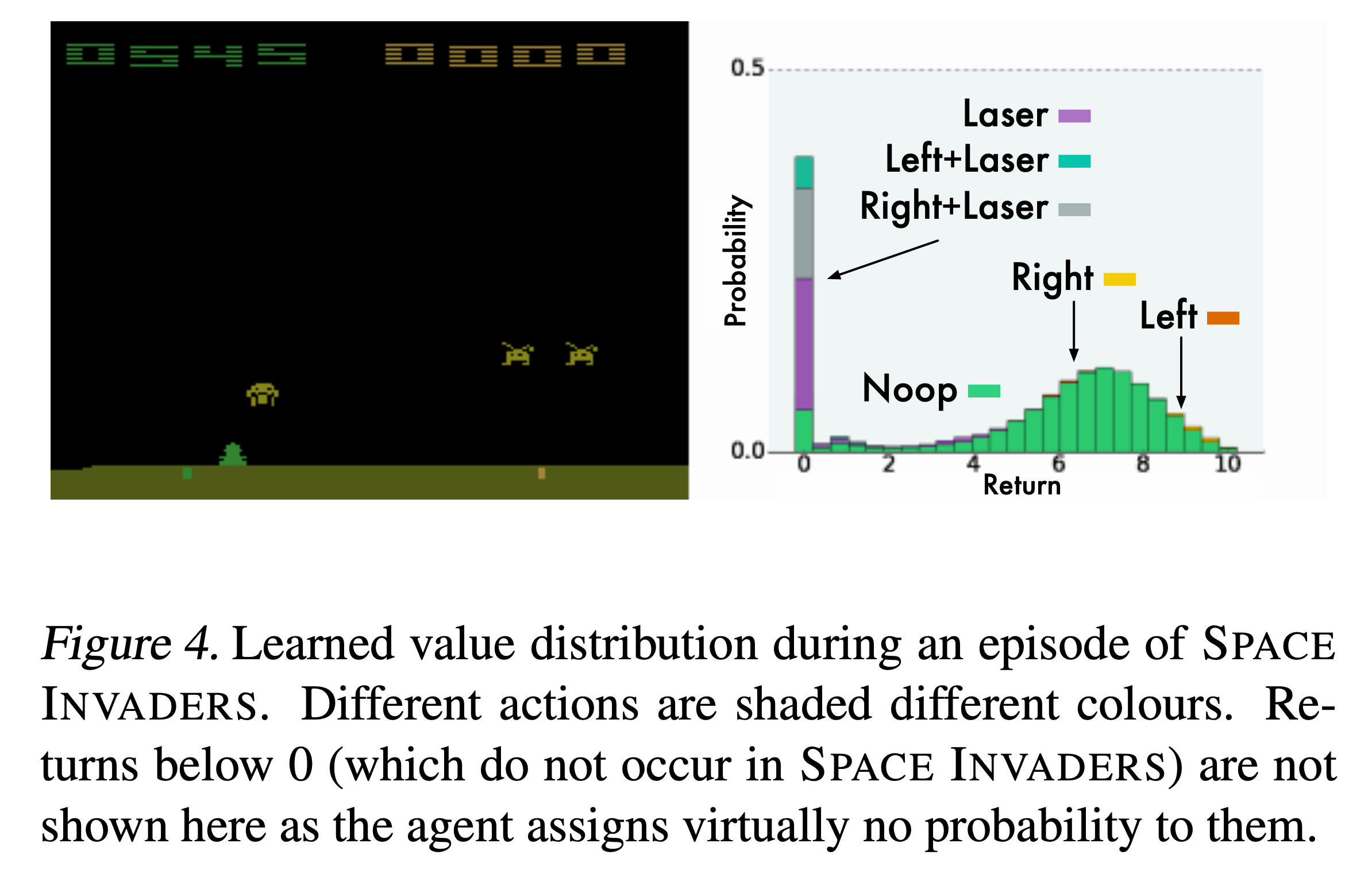 Fig.
Fig.
왼쪽 frame에서 그 다음 action으로 (Left+Lasor)를 할 경우 lasor를 너무 빨리 쏴서 죽을 것이기 때문에 0점에 delta function수준의 distribution이 형성된 걸 볼 수 있다 (그외 비슷한 action들도 모두 같음). 반면에 가만히 있거나? right, left로 가는 경우 distribution이 6~8쪽에 크게 분포해있는 걸 알 수 있다. 직관적으로 이 state에서 left, right를 했을 때 발생 가능한 trajectory들 중에 score가 높은 trajectory가 많을 것이라는 거다. 근데 위의 figure는 별 문제가 안 될 수 있지만, 만약 return distribution이 bimodal 혹은 multimodal이라면 어떻게 될까?
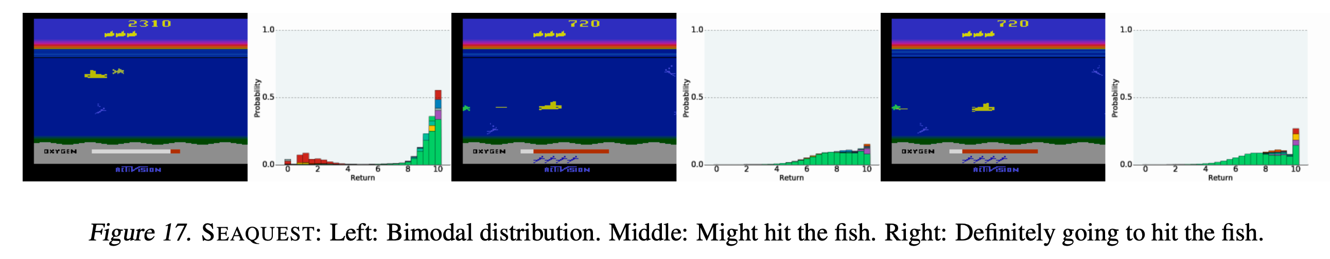 Fig.
Fig.
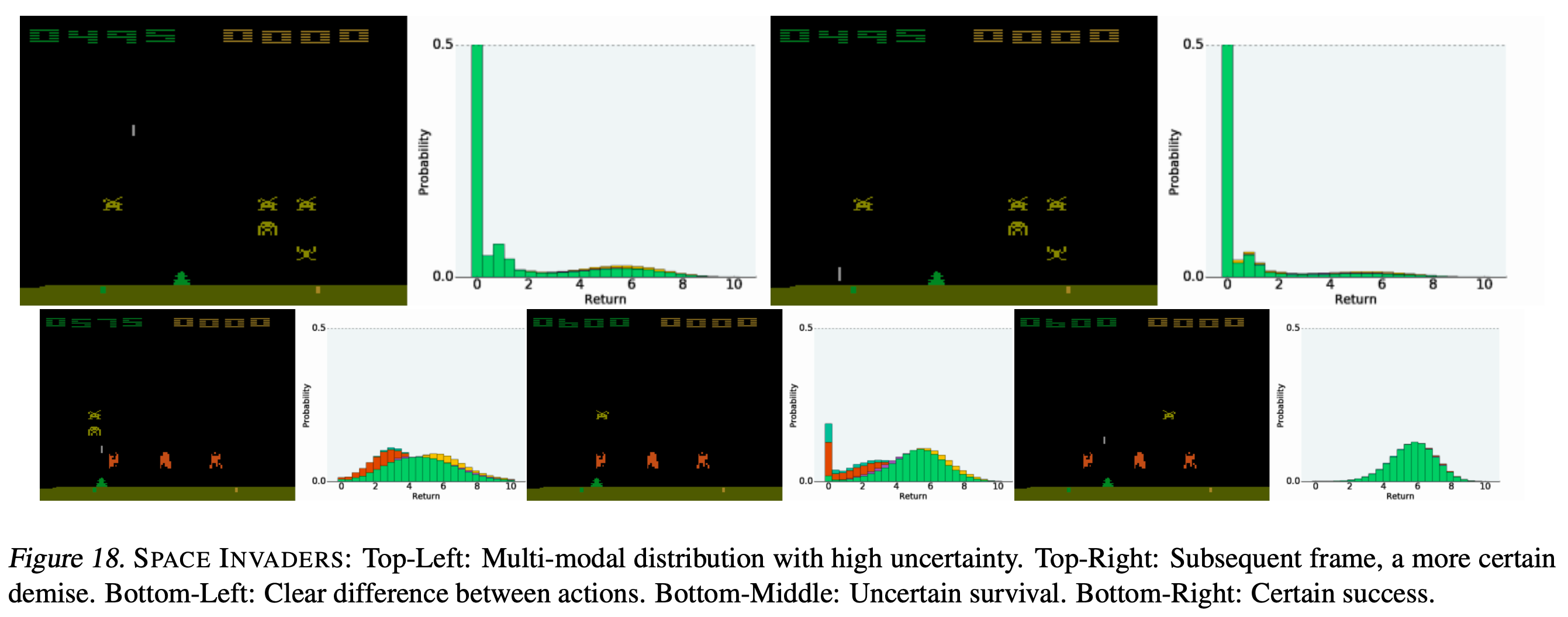 Fig.
Fig.
여기서부터는 이제 mean을 target으로 training과 inference를 하는 것이 문제가 될 수 있다. 실제로는 0점을 받을 trajectory가 많은데도 우연히 성공한 trajectory가 좀 있다고 해서 4~5점의 mean값으로 그 action을 평가하는건 문제가 있지 않을까? 실제로 \(Q(s_t,a_t)\)는 아래와 같이 계산되는데,
\[Q(s_t,a_t) = \sum_i P_w (Z(s_t,a_t = z_i )) \cdot z_i\]여기서 \(z_i\)는 발생가능한 trajectory중 i번째 trajectory의 return을 말하고 C51은 이를 weighted sum하는 식으로 action을 평가하게 되는데, 이것이 더 정확한 expectation을 계산할 수 있게 해준다고 한다.
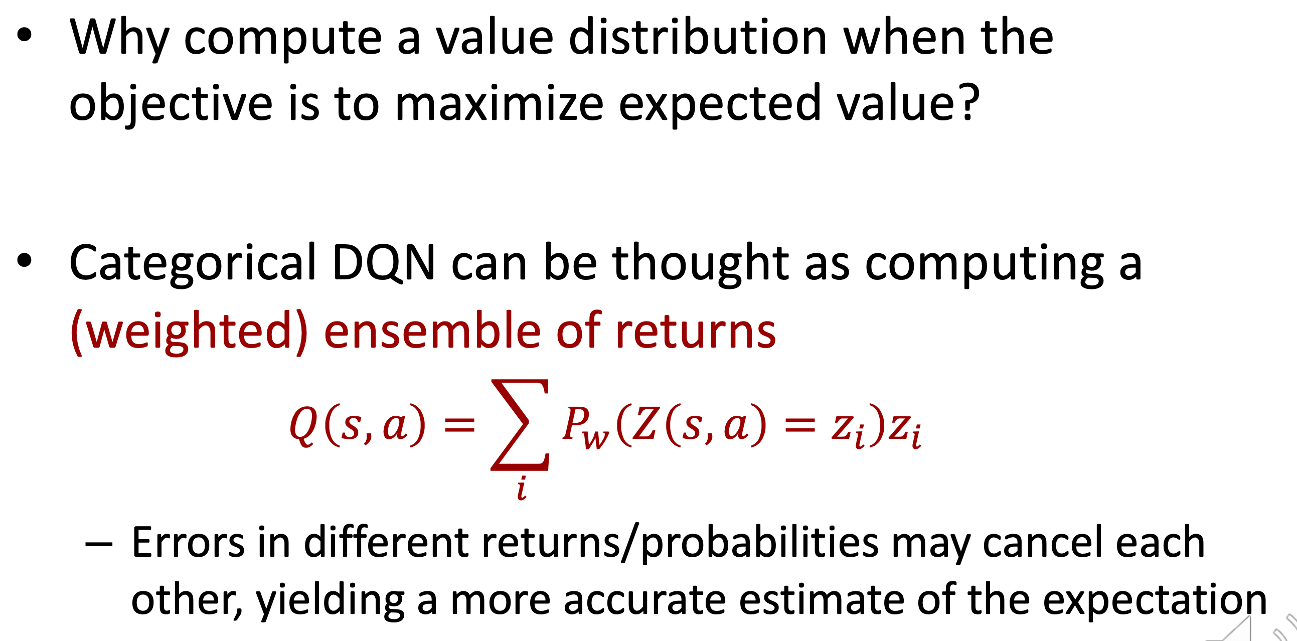 Fig.
Fig.
From a supervised learning perspective, learning the full value distribution might seem obvious:
why restrict ourselves to the mean?
The main distinction, of course, is that in our setting there are no given targets.
Instead, we use Bellman’s equation to make the learning process tractable;
we must, as Sutton & Barto (1998) put it, “learn a guess from a guess”.
It is our belief that this guess work ultimately carries more benefits than costs.
Categorical DQN with 51 Category (C51)
Q-Learning의 원래 goal은 expected current reward와 random transition으로 인해 미래에 얻게될 return의 expectation (expected outcome)의 합을 regression하는 것이다.
\[Q^{\pi}(s,a) = \mathbb{E} [R(s,a)] + \gamma \mathbb{E}_{P, \pi} [Q^{\pi}(s',a')]\]여기서 \(\pi\)는 Q값으로부터 유도된 policy이고 \(P\)는 transition matrix, \(R\)은 reward function 혹은 reward distribution이다. 보통 Q-learning을 한다고 치면 current reward는 어떤\(s\)에서 \(a\)를 하는 순간 environemnt가 주기 때문에 scalar를 쓰지만, 지금은 이를 probability distribution으로 정의하고 있다. 왜냐면 같은 state에서 같은 action을 하더라도 environment의 stochasticity가 존재하기 때문에 reward가 달라질 수 있어 이것이 자연스럽지만 DQN등에서는 이를 sampling으로 쓴 것이라 할 수 있다.
C51의 goal은 expectation이 Q값인 어떤 random return, \(Z\)를 학습하는 것인데,
이것또한 Q값을 bellman equation (recursive equation)으로 표현하듯 아래와 같이 표현할 수 있으며,
이를 Distributional Bellman Equation이라고 정의한다.
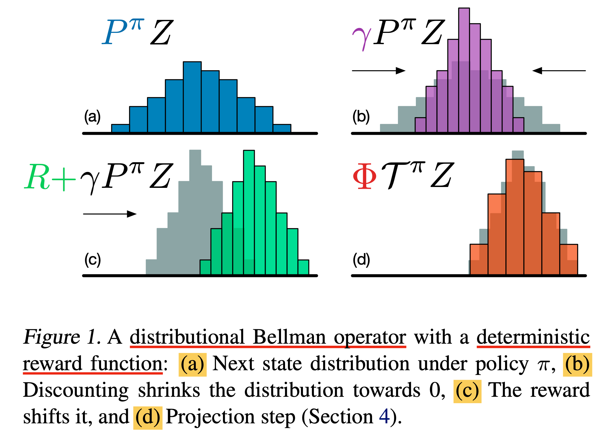 Fig.
Fig.
 Fig.
Fig.
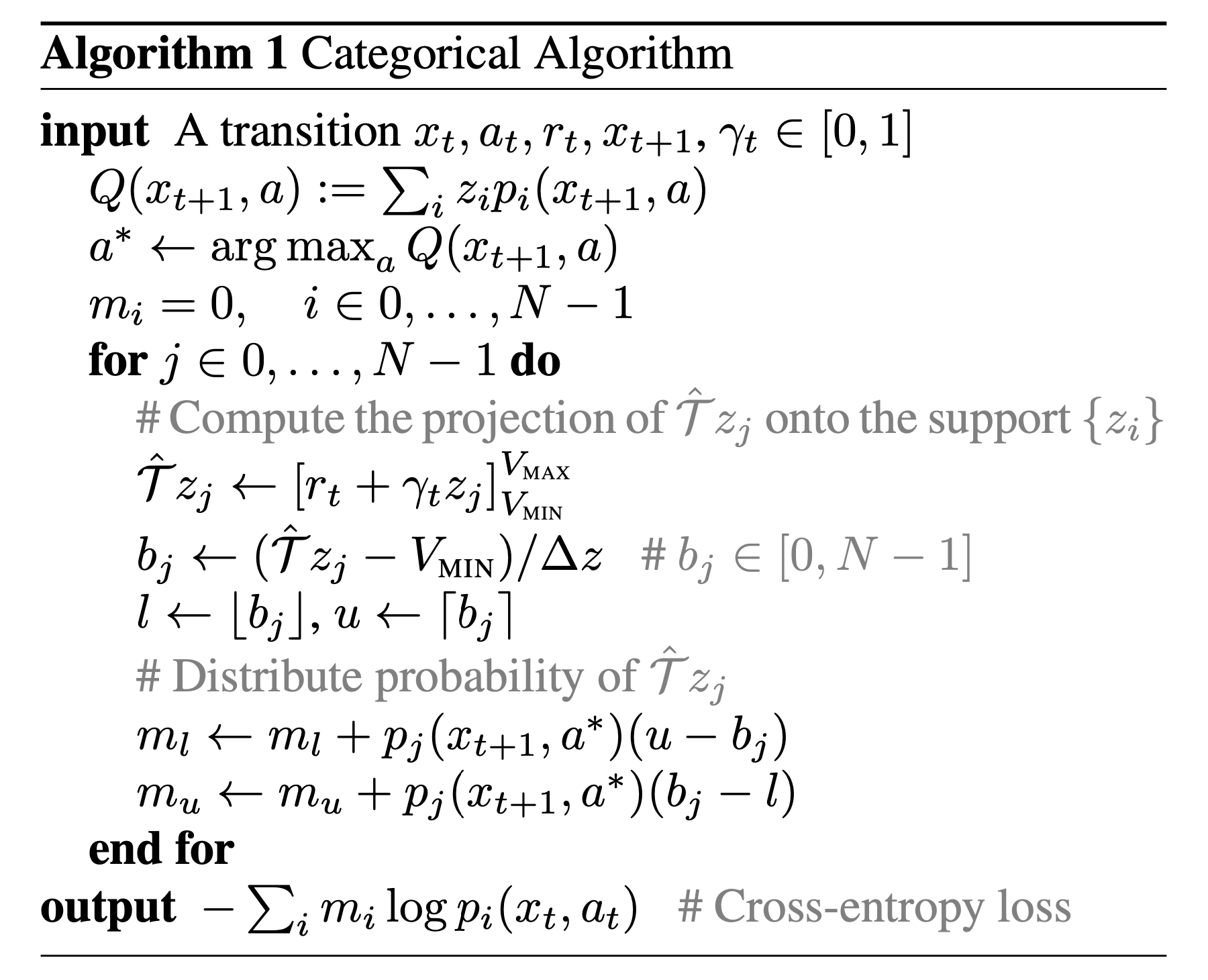 Fig.
Fig.
 Fig.
Fig.
Quantile Regression DQN (QR-DQN)
 Fig.
Fig.
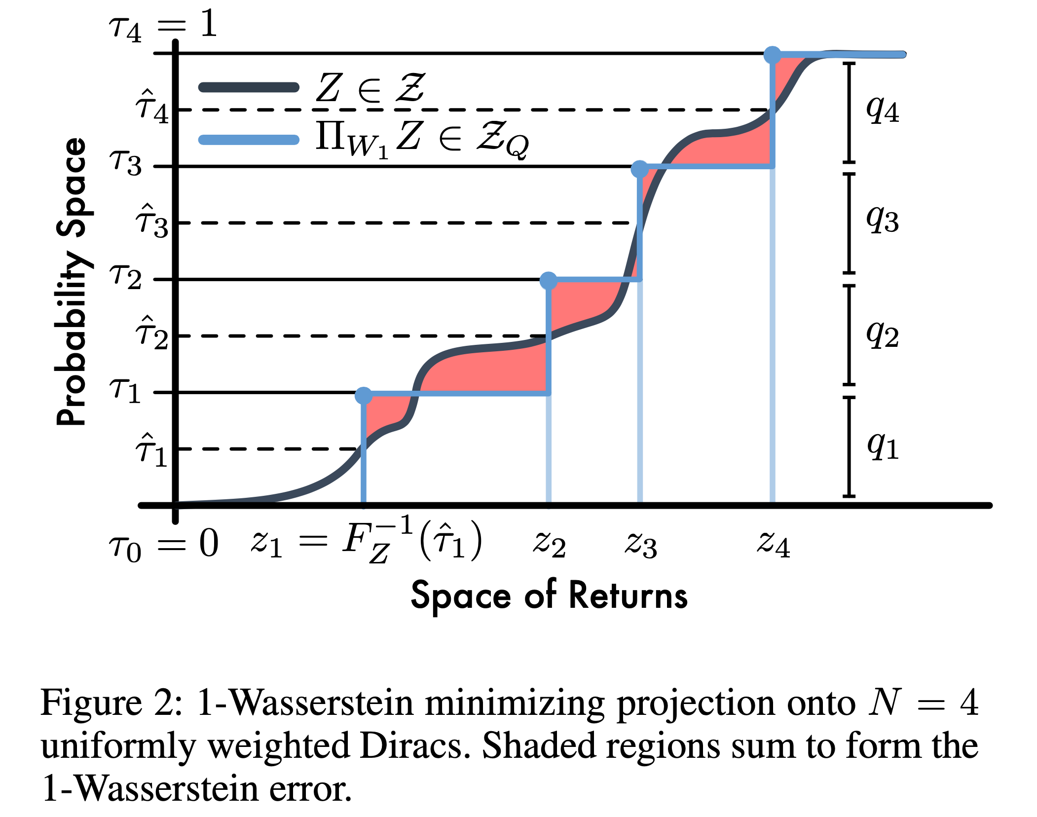 Fig.
Fig.
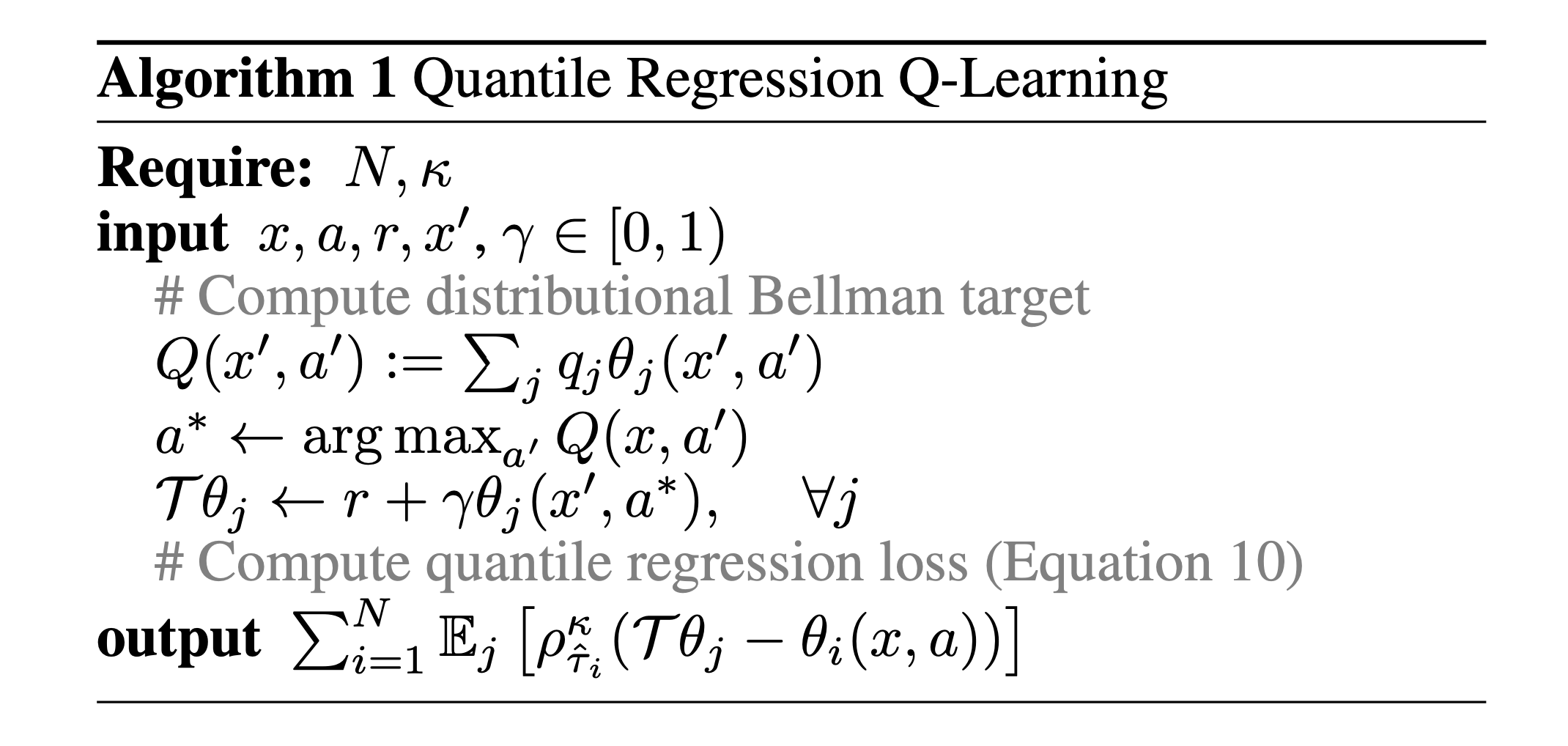 Fig.
Fig.
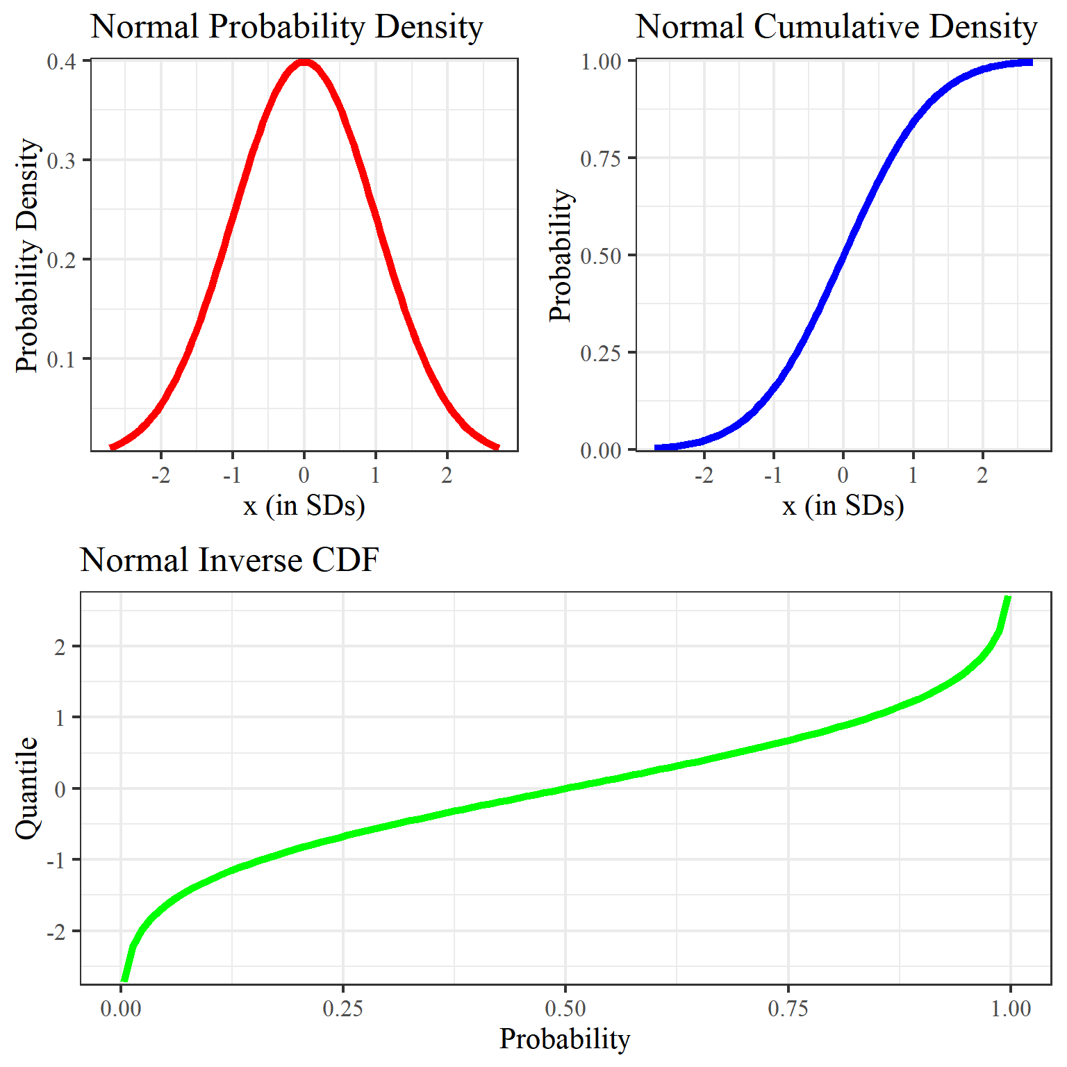 Fig. Probability Density Function (PDF), Cumulatve Distribution Function (CDF) and Quantile Function/Inverse Cumulative Distribution Function. Source from here
Implicit Quantile Network (IQN)
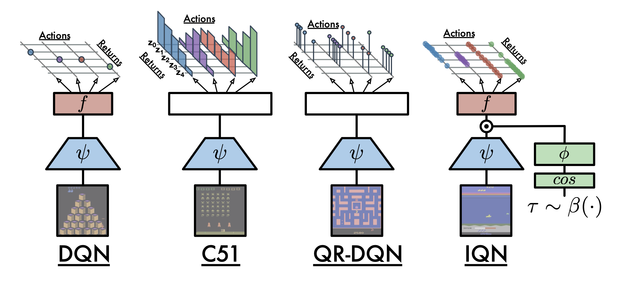 Fig.
Fig.
References
- Papers
- Others
- Codes