(WIP) Off-Policy RL
08 Aug 2023< 목차 >
Why Off-policy ?
Off-policy algorithm이 등장한 가장 큰 이유는 무엇일까?
일반적인 Reinforcemet Learning (RL) algorithm 들은 모두 On-policy method들인데 (Actor-Critic, PPO), 이들의 가장 큰 단점은 매 optimization step 마다 data를 새로 sampling 해야 된다는 것이다.
다시 말해 이전 trajectory (old data)들은 필연적으로 버려야 하는데 그 이유는 수학적으로 gradient를 계산할 때 \(k\)시점의 current policy, \(\pi_k\)가 만든 data를 써야 하기 때문이라고 한다.
그 결과 on-policy algorithm들은 Sample Inefficiency 하다고 많이 얘기하는데, 이는 good policy를 얻기 위해 얼마나 많은 sample이 필요한가?를 얘기한다.
일반적으로 사람은 바둑을 두는 모습을 보고 대충 룰을 파악하고 기본적인 수를 두는 데 몇 분 밖에 안걸리겠지만 RL algorithm들은 그렇지 수십~수백만 sample을 통해 학습해야 하는데 이를 sample inefficient하다고 한다.
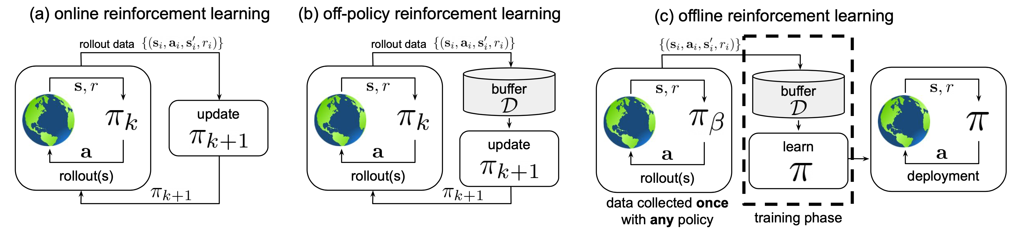 Fig. Online (On-policy) vs Off-policy vs Offline RL.
그렇다면 off-policy algorithm은 어떨까? 이는 무엇이고 이런 류의 algorithm의 sample efficiency는 어떠한가?
RL이란 \(k\)시점의 current policy, \(\pi_k\)가 trajectory를 sampling하고 이 trajectory내의 state, action pair를 보고 “이 state에서 이 action은 과연 좋았나?”를 environment와의 interaction을 통해 평가 (Reward)받고 좋았던 action은 확률을 높히는 방향으로, 아닌 action은 줄이는 방향으로 policy를 학습한다.
즉 일반적인 RL (online, on-policy)의 경우 trajectory data를 만드는 policy를 behavior policy라고 하는데 이것이 current policy라는 것이고, 내가 학습하고자 하는 policy를 target policy라고 하는 이것 또한 current policy가 되는 것이다.
하지만 off-policy의 경우 behavior를 하는 policy와 내가 학습하고자 하는 target policy가 다른데, 즉 다른 policy가 만들어놓은 data를 쓸 수 있다는 의미다.
- Key elements
- Behavior Policy : trajectory를 만들어주는 policy (\(\pi_{\beta}\))
- Traget Policy : 학습하려는 policy (현재 \(k\)시점의 policy, \(\pi_k\))
- On-policy : \(\pi_k = \pi_{\beta}\)
- Off-policy : \(\pi_k \neq \pi_{\beta}\)
이는 예를 들어 바둑을 두는 agent를 만들고 싶은데 이세돌 9단이 둔 기보 data나 alphago의 기보 data를 사용하는것을 말한다. 초기상태의 허접한 policy를 생각해보면 배운게 없을테니 아무 action이나 하라는 decision을 할텐데 이렇게 아무 action이나 한 trajectory를 또 허접한 policy가 평가를 해야 하는 것이니 얼마나 학습이 오래걸릴까? (sample inefficiency)
## The On-Policy Algorithms (VPG, TRPO, PPO and so on)

they don’t use old data, which makes them weaker on sample efficiency.
But this is for a good reason: these algorithms directly optimize the objective you care about—policy performance—
and it works out mathematically that you need on-policy data to calculate the updates.
So, this family of algorithms trades off sample efficiency in favor of stability—
but you can see the progression of techniques (from VPG to TRPO to PPO) working to make up the deficit on sample efficiency.

## The Off-Policy Algorithms (DDPG, Q-Learning and so on)

Algorithms like DDPG and Q-Learning are off-policy, so they are able to reuse old data very efficiently.
They gain this benefit by exploiting Bellman’s equations for optimality,
which a Q-function can be trained to satisfy using any environment interaction data
(as long as there’s enough experience from the high-reward areas in the environment).
But problematically, there are no guarantees that doing a good job of satisfying Bellman’s equations
leads to having great policy performance.
Empirically one can get great performance—and when it happens,
the sample efficiency is wonderful—but the absence of guarantees makes algorithms in this class potentially brittle and unstable.
TD3 and SAC are descendants of DDPG which make use of a variety of insights to mitigate these issues.
Source from link
한편 RL method를 구분지을 때 Online vs Offline RL로 나누기도 하는데, Offline RL은 environment와 interaction이 전혀 없이 맨처음에 모은 trajectory sample들만 가지고 학습하는데 이 sample들은 이미 학습된 agent나 human expert의 simulation trajectory들인 경우가 대부분이다.
tmp
본 Post에서는 on-policy와 off-policy의 차이에 대해 알아볼 것이며 어떤상황에서 무엇이 더 좋은지 까지 논의해 보려고 한다.
Experience Replay
Exploration
Some Algorithms
Soft Actor-Critic (SAC)
Vanilla Actor Critic 은 on-policy RL을 가정하고 만들어졌다.
이를 off-policy manner로 쓰려고 보완한 것이 바로 Soft Actor Critic (SAC) 이다.
SAC의 핵심은 entropy regularization으로 policy의 가 얼마나 random한가?를 의미하는 entropy와 sum of expected reward간의 trade-off를 최대화 하도록 학습된다.
RL의 핵심 요소인 exploration-exploitation trade-off와도 밀접한 관계가 있다고 하는데, entropy는 exploration을 강화하여 더 많은 수를 봄으로써 나중의 학습 속도를 가속화 하거나 조기에 잘못된 local minima에 빠지는 것을 막아준다고 한다.
Entropy의 개념부터 보도록 하자. 이는 다음의 수식으로 계산되며 얼마나 확률 분포가 random한가를 나타낸다.
\[H(P) = \mathbb{E}_{x \sim P} [ - \log P(x) ]\]RL의 Objective 를 다시 보자. 우리가 어떤 policy를 따랐을 때 받을 총 reward의 합의 기대값이 최대가 되도록 policy를 학습하는 것이 모든 RL의 궁극적인 목표이다.
\[\begin{aligned} & J(\pi) = \int_{\tau} P(\tau \vert \pi) R(\tau) = \mathbb{E}_{\tau \sim \pi} [ R(\tau) ] & \\ & \pi^{\ast} = \arg \max_{\pi} J(\pi) \\ \end{aligned}\]Reward function을 time-step별로 풀어쓰면 다음과 같은데,
\[\pi^{\ast} = \arg \max_{\pi} \mathbb{E}_{\tau \sim \pi} [ \sum_{t=0}^{\infty} \gamma^t R(s_t, a_t, s_{t+1}) ]\]여기에 매 step별로 bonus reward를 주는 것이 기본 idea이다.
\[\pi^{\ast} = \arg \max_{\pi} \mathbb{E}_{\tau \sim \pi} [ \sum_{t=0}^{\infty} \gamma^t (R(s_t, a_t, s_{t+1}) + \color{red}{ \alpha H(\pi(\cdot \vert s_t)) } ) ]\]이 bonus는 entropy 크면 좋은것이기 때문에 policy의 distribution이 평평할수록 (peak하지 않을수록) 좋은 것이며 \(\alpha>0\)는 trade-off coefficient이다.
이제 Value Function, V도 다시 정의해보자 (우리는 결국 Actor-Critic form을 유도해야 하므로). 만약 어떤 state, s에서 agent가 출발한다면 V는 다음과 같다.
\[V^{\pi}(s) = \mathbb{E}_{\tau \sim \pi} (R(\tau) \ vert s_0 = s)\]여기에도 entropy bonus를 포함시키면 다음과 같은 수식을 얻를 수 있다.
\[V^{\pi}(s) = \mathbb{E}_{\tau \sim \pi} [ \sum_{t=0}^{\infty} \gamma^{t} ( R(s_t, a_t, s_{t+1}) + \color{red}{ \alpha H(\pi(\cdot \vert s_t)) } ) \vert s_0 = s]\]Action-Value Function인 Q도
\[Q^{\pi}(s,a) = \mathbb{E}_{\tau \sim \pi} [ R(\tau) \vert s_0=s, a_0=a ]\]다음처럼 변해야 한다.
\[Q^{\pi} (s,a) = \mathbb{E}_{\tau \sim \pi} [ \sum_{t=0}^{\infty} \gamma^t R(s_t, a_t, s_{t+1}) + \color{red}{ \alpha \sum_{t=0}^{\infty} \gamma^{t} H(\pi(\cdot \vert s_t)) } \vert s_0 = s, a_0 = a ]\]위의 정의들에 따라서 V는 다음과 같이
\[V^{\pi}(s) = \mathbb{E}_{a \sim \pi} [ Q^{\pi}(s,a) ] + \alpha H(\pi (\cdot \vert s))\]가 되며 Q에 대한 bellman equation은 다음과 같이 정리된다.
\[\begin{aligned} & Q^{\pi}(s,a) = \mathbb{E}_{s' \sim P} [ R(s,a,s') + \gamma ( Q^{\pi}(s',a') + \alpha H(\pi (\cdot \vert s') ) ] & \\ & = \mathbb{E}_{s' \sim P} [ R(s,a,s') + \gamma V{\pi} (s') ] \\ \end{aligned}\]이제 이
 Fig.
Fig.