(WIP) Rescent Advances in Deep Generative Model (1/4) - Diffusion Model

< 목차 >

• Diffusion Model as Latent Variable Model
  • Is DDPM a kind of VAE?
• TLDR; Diffusion Model
  • Forward (Diffusion) Process (Adding Noise)
  • Reversed Process (Denoising Process)
  • Training Objective (ELBO, Noise Prediction)
  • Training Algorithm
  • Inference Algorithm
  • Model Architecture
  • Results
  • tmp
• References

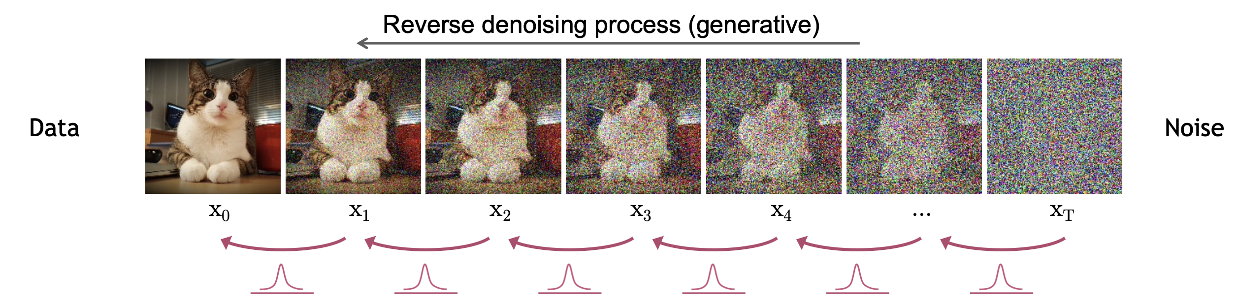
확산 기반 생성 모델 (Diffusion-based Generatvie Model) 이 이미지 생성 (Image Synthesis) 분야를 집어 삼키고 있습니다. 주어진 text (description, prompt) 을 바탕으로 원하는 이미지를 만들어내는Text-to-Image (T2I), 원본 이미지를 주고 편집 (edit) 하고 싶은 부분에 대한 묘사 (prompt or image) 를 해주면 이를 기반으로 이미지를 번역해주는 Image Translation 이나 Inpainting 등에서도 놀라운 결과를 보여주고 있는데요, diffusion 기반 Open-Source 모델을 custom해서 월마다 정기 구독 시템ㅡ로 돈을 쓸어담는 스타트업까지 나타나고 있습니다.

Fig. Diffusion-based Generative Model 의 작동 방식. Source from here

본 Post 에서는 Diffusion-based Models 의 원리가 뭐길래? 왜 이 모델은 기존의 방식들과 다르게 고 퀄리티 (High Fidelity) 이미지를 만들고, 이미지를 원하는 의도 대로 만들 수 있는 Controllability 가 뛰어난 것인지에 대해 다뤄보려고 합니다.

Diffusion Model as Latent Variable Model

Diffusion Model 은 뭘까요? Diffusion Model은 VAE와 같은 잠재 변수 (Latent Variable) 기반의 생성 모델로 분류됩니다. 과연 이 둘은 어떤게 비슷하고 다를까요?

VAE는 가우시안 분포 같은 간단한 분포에서 noise를 샘플링 하고 이를 이미지로 Decoding 하도록 Encoder, Decoder를 학습하는 반해

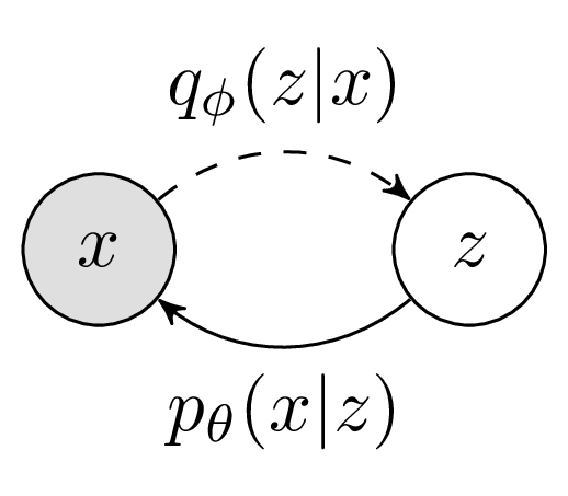Fig. VAE 의 Graphical Model. Source from here

Diffusion Model은 아래와 같이 여러번에 걸쳐 노이즈로부터 이미지를 만들어냅니다. 즉 VAE 같은 latent variable 모델을 여러번 거치는 확장판이라고 생각해볼 수 있습니다.

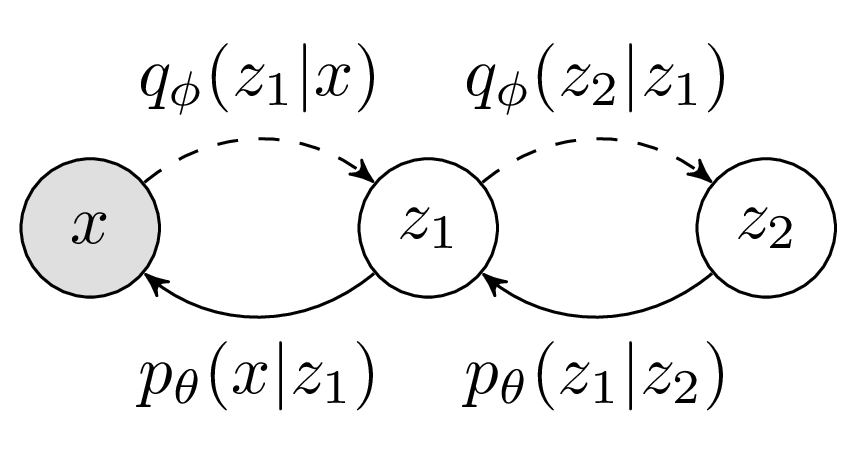Fig. Hierachical VAE. Source from here

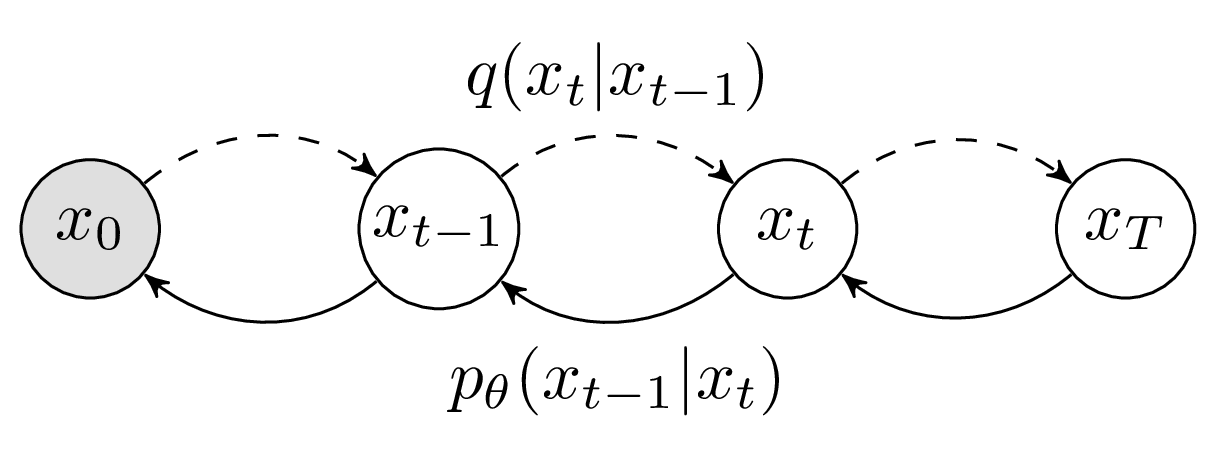Fig. Diffusion Model. Source from here

DDPM 이라는 Diffusion 기반 approach의 core paper에서는 아래의 그림으로 Diffusion Model을 표현했는데요

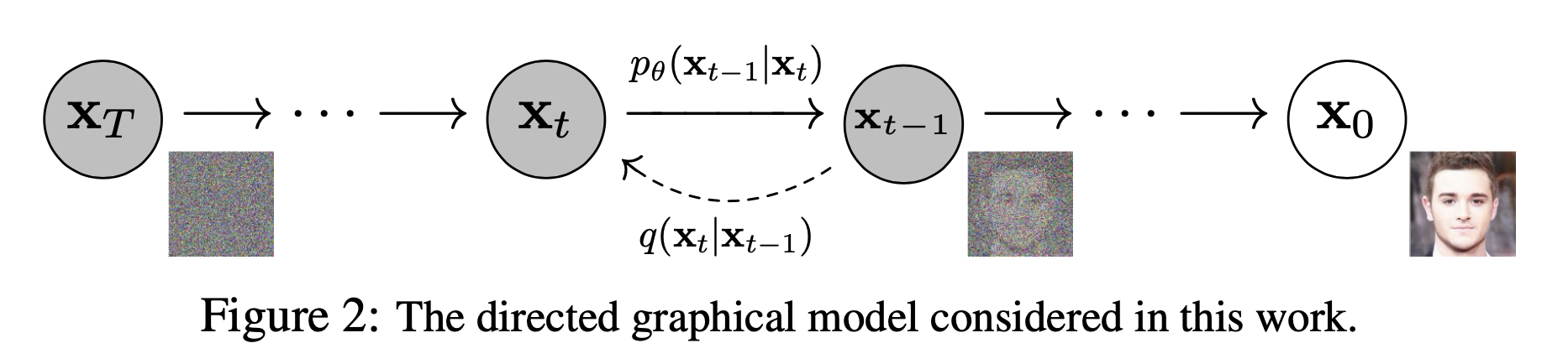Fig. 논문에서 묘사한 diffusion model의 graphical model

위의 그림을 보면 맨 왼쪽 (white noise) 부터 시작해서, \(\theta\)로 parametrized 된 model이 이를 점점 이미지 처럼 변환시켜 주는 걸 알 수 있습니다.

그런데 잠재 변수 모델 (latent variable model)은 뭘까요?

기본적으로 Machine Learning은 \(p(x), p(x \vert y), p(y \vert x)\)같은 likelihood를 를 최대화 하는 Maximum Likelihood 를 최적화 합니다. 이 중에서 \(p(x), p(x \vert y)\)같은 input에 대한 분포를 modeling하는 것을 생성 모델 (generative model) 이라고 합니다. 그런데 이 중에서 \(p(x)\)를 modeling하는 것은 우리가 가지고 있는 데이터가 input의 정보, 즉 image pixel 값들로 이루어진 sample \(x\)들이 어떤 분포에서 sampling됐을까? 를 modeling하는 것이 됩니다. 그런데 이 사진들에 각각 숨겨진 정보가 있을 수 있고 이는 개, 고양이라는 class label이 될 수도 있고 이를 \(z\)라고 합니다.

이 \(z\)라는 변수는 숨겨졌기 때문에 잠재된 (latent)라는 말을 쓰고, 잠재 변수 모델은 보통 우리가 실제로 알 수는 없지만 (데이터에는 없지만) 존재한다고 가정하는 \(z\) 라는 잠재 변수를 넣어서 \(p(x) = \int p(x \mid z) p(z) dz\) 라는 분포를 최대화 하는 문제를 풀게 됩니다.

이렇게 하는 이유는 원래 굉장히 복잡한 분포 \(p(x)\) 를 modeling하는 문제를 두 개의 간단한 분포로 나눠서 풀게해줍니다.

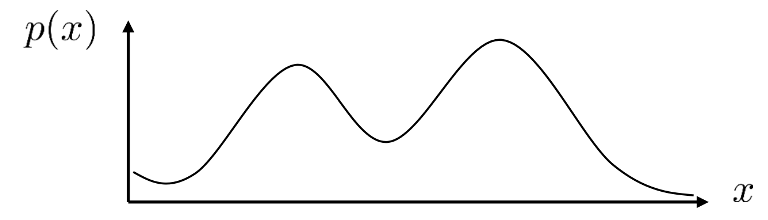Fig. 굉장히 복잡한 원본 분포

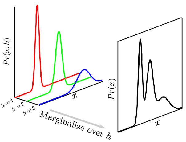Fig. 잠재 변수를 넣으면 복잡한 분포를 모델링하기 쉽다. 잠재 변수 = h (z라고도 쓴다)

이런 잠재 변수 model 대표적인 Application 중에 Variational AutoEncoder (VAE) 를 예로 들 수 있는데, 이는 말씀드린 것 처럼 복잡한 \(p(x)\)를 modeling하기 위해서 latent variable을 도입하면서 AutoEncoder 구조를 차용함으로써

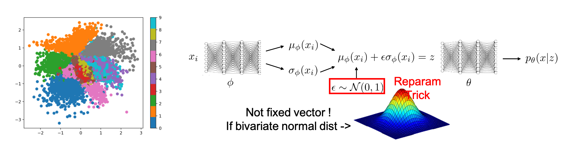Fig. VAE의 모식도

Latent Space 에서 Noise Vector 를 랜덤 샘플링 해서 decoding하는 것으로 새로운 data를 만들어 내는 (sampling) 알고리즘 입니다.

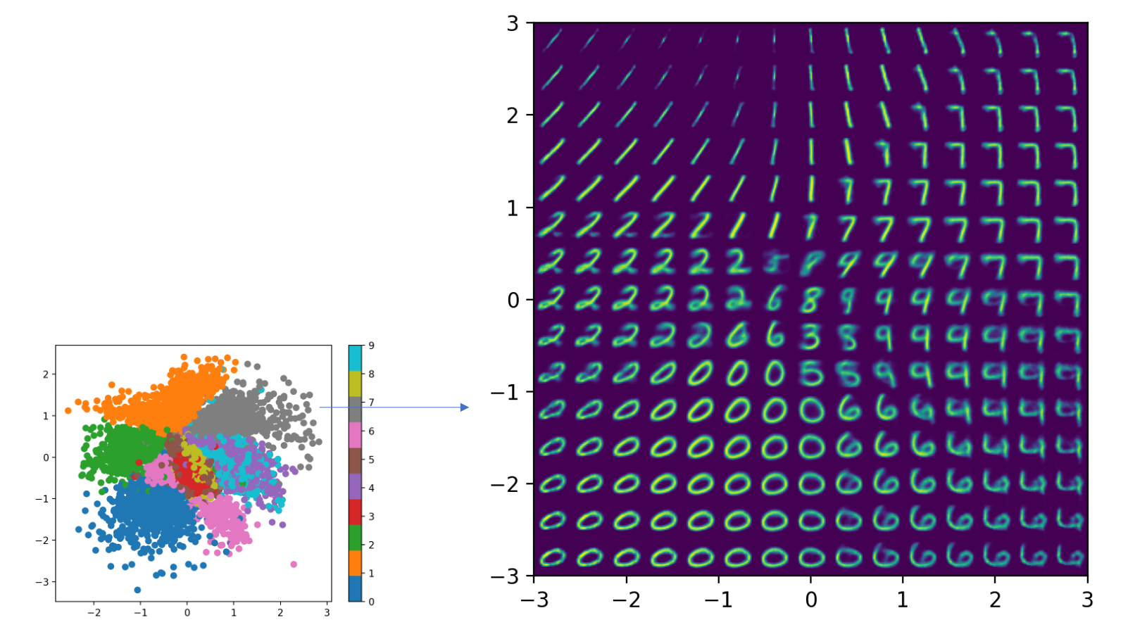Fig. VAE 의 이미지 샘플링 (생성)

Is DDPM a kind of VAE?

Angus Turner는 본인의 Blog에 DDPM이 VAE와 어떤면에서 유사한점과 차이점이 있는지 자신의 insight를 적어두었는데요, 두 모델은 다음 세 가지의 유사한 점을 가지고 있다고 합니다.

• 1.We have a generative model (the reverse process) that involves sampling some latent variable and transforming it into data with a neural network
• 2.We have a corresponding inference model (the forward process), which transforms data into a series of latent representations.
• 3.The training objective is a lower bound on the data likelihood, which can be derived in a similar fashion to the VAE.

반면에 다음 네 가지의 차이점이 두 모델을 구분짓는다고 합니다 (논문에도 Diffusion Model이 다른 Latent Variable Model과 다른 점에 대해 저자의 코멘트가 있긴 합니다).

• 1.The inference model or forward process in DDPM has no learned parameters
• 2.The forward process in DDPM progressively destroys all information about the input, such that the final distribution \(q(x_T \mid x_0)\) is a standard gaussian by construction. This is typically not true with VAEs (we want \(z\) to contain some information about \(x\) !)
• 3.In DDPM the dimensionality of each latent must match the data. In VAEs we can reduce dimensionality.
• 4.In DDPM, each generative layer shares the same neural network parameters. This is not typical for VAEs, however it should be possible in theory (I am not sure if it has been explored).

TLDR; Diffusion Model

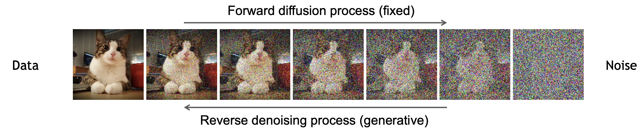
Diffusion Model을 수식적으로 이해하기 전에, 직관적으로 Diffusion 이 하고자 하는 일은 아래의 애니메이션과 같습니다.

Fig. 수차례의 Denoising 을 통해 고퀄리티 이미지를 만드는 Diffusion. Source from here

앞서 VAE같은 latent variable model이 결국 잘 학습되면 어떤 noise z로부터 image를 한번에 생성해 낼 수 있다고 했는데, diffusion model은 이 과정을 여러 개로 쪼갠 것으로 볼 수 있다고 말씀드렸죠. 그렇기 때문에 animation에서는 noise로부터 이미지가 서서히 만들어지는 겁니다.

Diffusion model의 이미지 생성 과정을 세 줄 요약하면 다음과 같습니다.

1. 이미지에 서서히 노이즈를 추가해 (T번 반복) 점점 완전히 노이즈만 남게 하는 식으로 이미지를 corrupt 한다.
2. t 번째 이미지에서 t-1 번 이미지로 가려면 어떤 노이즈를 빼줘야 할까? 를 모델이 예측하도록 학습한다.
3. T=1000 (예를 들어) 에서 부터 1000번 denoising 을 하면 고퀄리티 이미지를 샘플링 할 수 있다.

당연하게도 VAE를 여러번 한다는 부분에서 학습이 다 끝난 뒤에 이미지를 실제로 생성하는 과정에서 엄청난 comuputational cost가 예상되고 이를 풀기위한 Progressive Distillation같은 method들이 지속적으로 연구되고 있습니다. (LLM이고 이미지 생성쪽이고 간에 이 분야는 기업 입장에서도, end-user입장에서도 비용과 시간을 줄여주기 때문에 앞으로도 매우 유망할 것 같습니다.)

Forward (Diffusion) Process (Adding Noise)

이제 본격적으로 Diffusion model 에 대해 알아봅시다.

우리가 갖고있는 데이터는 \(x_0\) 라는 원본 이미지이고 이 이미지를 \(T\)번의 반복을 통해 더렵힌다고 생각해 봅시다. 이 때 마지막 T번째 이미지 \(x_T\)의 분포 \(p(x_T)\)는 아래와 같은 Gaussian 분포가 됩니다.

왜 그럴까요?

원본 이미지인 \(\mathbf{x}_{0}\) 는 \(\mathbf{x}_{0} \sim q\left(\mathbf{x}_{0}\right)\) 처럼 q 라는 분포 (데이터셋) 에서 샘플링 된 것입니다.

이를 어떻게 더럽히느냐? 가 궁금하실 텐데요, \(x_1\) 의 분포로 어떻게 가는지 먼저 생각해 봅시다.

먼저 \(x_0\) 라는 원본 이미지가 주어졌을 때 \(x_1\) 의 분포는

가 됩니다. (적분을 해보면 됩니다.)

이제 이를 t 번째에 대해 일반화 해 봅시다.

가 되는데요, 여기서 \(q(x_t \vert x_{t-1})\) 를 논문에서는 간단한 가우시안 분포로 정의하게 됩니다.

이는 단순히 이전 단계의 Image Vector인 \(\mathbf{x}_{t-1}\) 에 단순히 \(\sqrt{1-\beta_{t}}\) 를 곱해준 값을 mean으로 하고, \(\beta_t\) 크기의 동일한 Spherical Covariance 를 갖는 분포로 만드는 거죠.

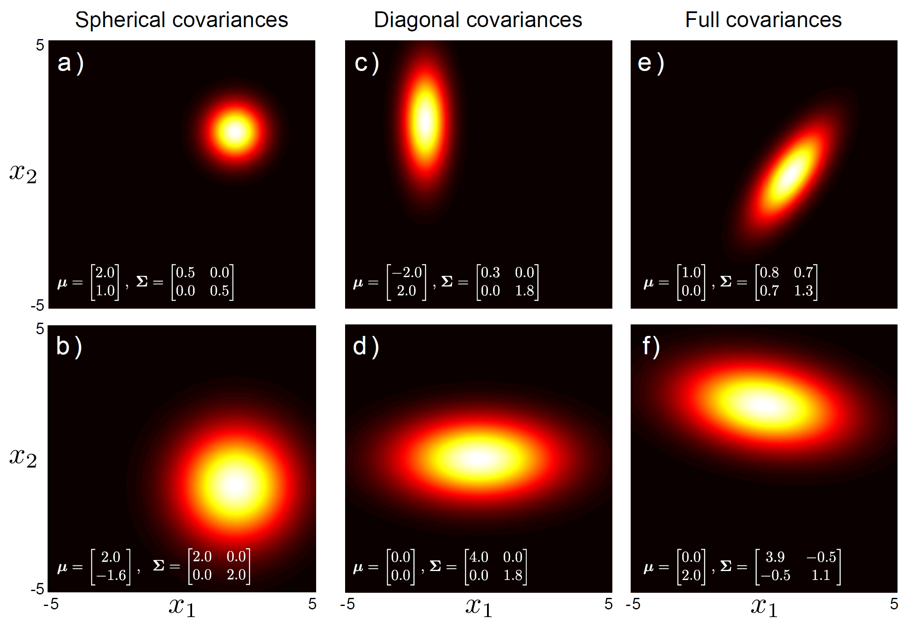Fig. Bivariate Gaussian Distribution with Various Covariances

이렇게 이미지에 점점 노이즈가 끼는 것을 Forward Process 혹은 Diffusion Process 라고 합니다.

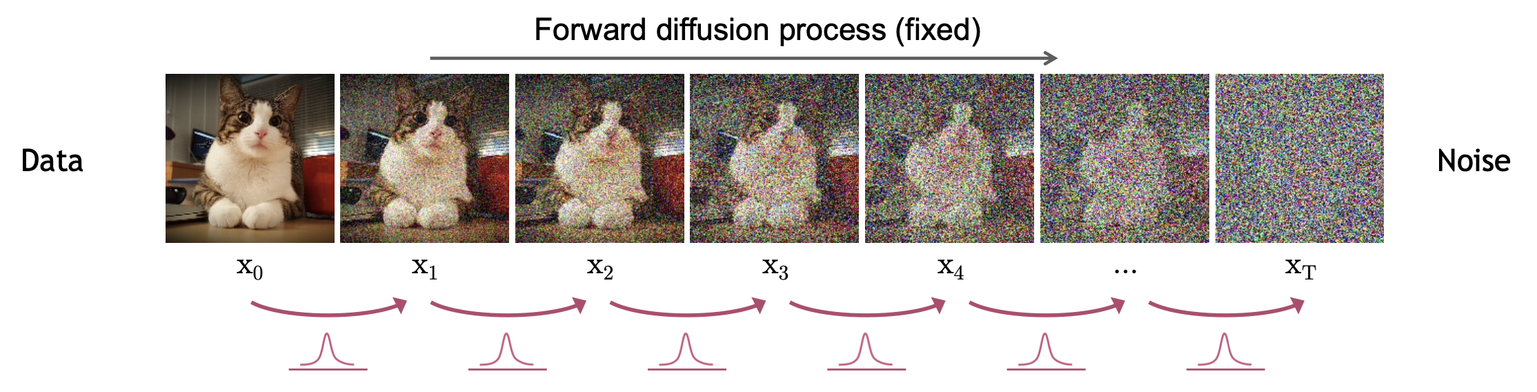Fig. Forward Process

그렇다면 \(x_0\) 원본 이미지를 T 번 더럽힌 경우는 어떻게 나타낼까요?

이는 Gaussian Diffusion Process 를 여러번 연산해준 것과 같은데요,

즉 T 번 이런 연산을 반복해준 것과 같고, 논문에서는 이를 아래와 같은 결합 분포로 나타냅니다.

로 표현할 수 있습니다. 여기서 보시면 \(x_{t}\) 을 만드는데 영향을 끼치는 건 \(x_{t-1}\) 뿐이라는 걸 알 수 있고 그 전 스텝의 \(x_{t-2}, \cdots, x_0\) 는 필요 없다는 걸 알 수 있는데요, 이런 조건 때문에 Diffusion Model은 Markov Chain이라고 할 수 있습니다.

그렇다면 \(x_t\) 의 corrupted sample를 만드는 데 반드시 \(x_{t-1}\) 이 필요할까요? 그렇지 않습니다. Markov Property 가 있지만 우리가 Forward Process 를 가우시안 으로 정의했기 때문에 \(x_0\) 로 부터 단번에 \(x_t\) 를 샘플링 할 수 있는데요,

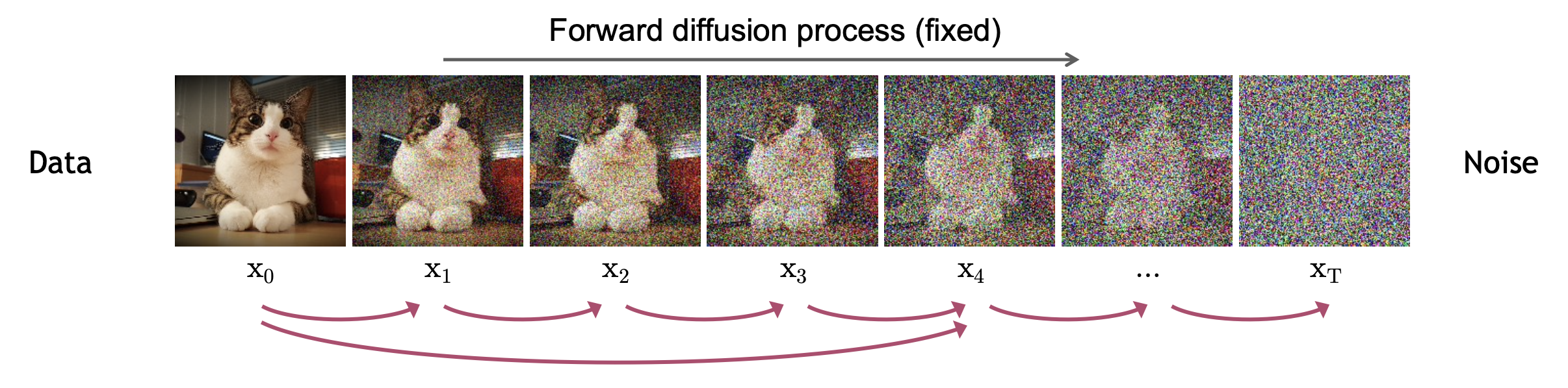
이는 아래의 수식을 사용하면 되고

이 때 \(\alpha\) 는 \(\beta\) 를 이용한 값이 됩니다.

여기서 \(\beta_t\) 값은 1보다 작은 값인데요, 즉 이 값이 여러번 곱해진 \(\alpha\) 는 0에 가까운 값을 나타내게 되며 바로 이 때문에 \(x_T\) 는 0 (zero) mean 1 (unit) variance 의 가우시안 분포가 되는 것입니다.

한편 이렇게 \(x_0\) 에서 \(x_{t-1}\) 로 가는 관계식을 알게 됨으로써 우리는 아래의 수식을

아래처럼 재 정의할 수 있습니다.

이렇게 원본 이미지의 분포와 디퓨전 커널 (Diffusion Kernel) 를 적분하는 과정을

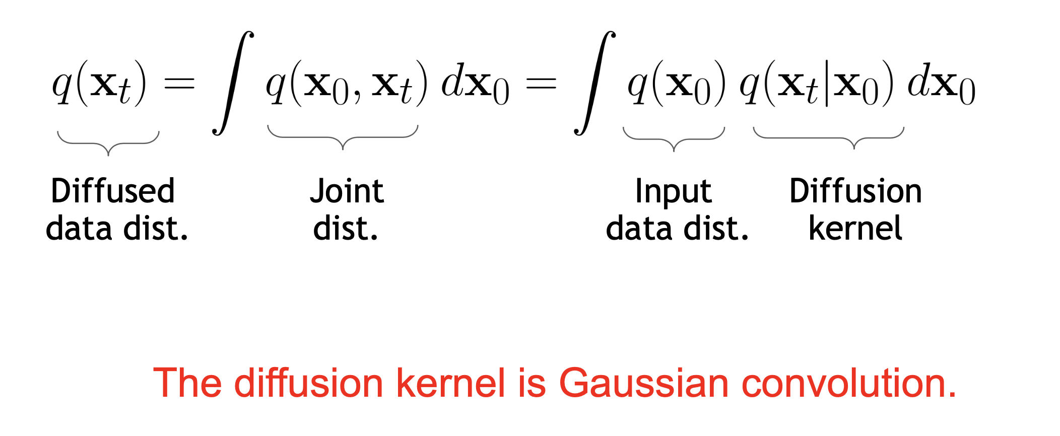
Gaussian Convlution 이라고 할 수 있는데요, 우리가 원하는 건 \(q(x_t)\) 의 분포 까지는 아니고 결국 이로부터 샘플링한 이미지 \(x_t \sim q(x_t)\) 이므로 \(x_0 \sim q(x_0)\) 를 먼저 하고 (원본 데이터를 뽑고) \(x_t \sim q(x_t \vert x_0)\) 를 하면 t 번 더럽혀진 이미지를 샘플링할 수 있게 됩니다.

여기서 주의할 점 (?) 은 가우시안 형태의 커널이 점진적으로 Convolution 되면서

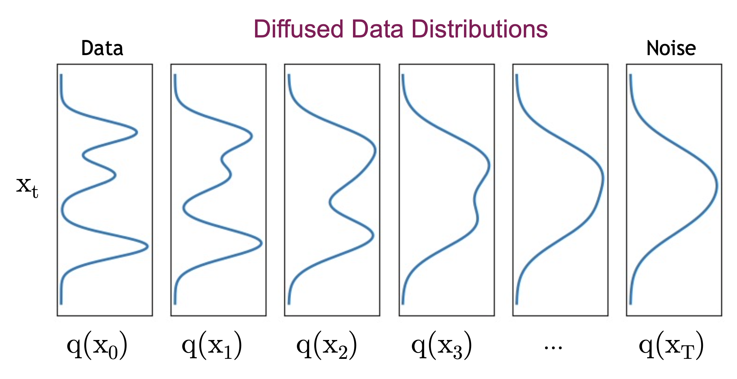
점차 가우시안에 가까운 분포가 되긴 하지만 \(q(x_1), q(x_2), \cdots\) 의 분포들이 모두 가우시안이냐? 는 아니라는 겁니다.

마지막으로 디퓨전 커널을 Convolution 해주는 Forward Process 는 사실상 Gaussian Noise를 이미지에 추가하는 것이라고 볼 수 있다고 논문에서는 표현하고 있습니다. (아마 수식적으로도 그럴 겁니다 (…?))

(In Paper)

forward process or diffusion process, is fixed to a Markov chain that gradually adds Gaussian noise to the data according to a variance schedule β1 , . . . , βT

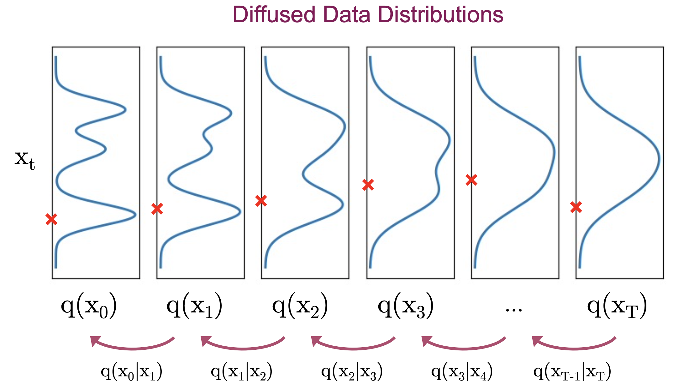
Reversed Process (Denoising Process)

이번에는 반대로 생각해볼까요?

우리가 원하는 건 사실 반대 과정인 Reversed Process 니까요.

다시, T번 더럽혀진 이미지는 \(q(x_T) \approx N(x_t ; 0, I)\) 였습니다.

우리가 원하는 일은 T 번째 이미지

를 최초로 샘플링 하고 T 번 반복적으로 Denoising 된 이미지를 샘플링 하는 겁니다.

이 때 \(q\left(\mathbf{x}_{t-1} \mid \mathbf{x}_t\right)\) 를 실제 분포인 True Posterior (Denoising Distrubition) 라고 합니다.

하지만 대부분의 경우 이를 계산하는 건 현실적으로 불가능 (intractable) 한데요,

그렇기 때문에 이를 근사한 approximate posterior 를 정하고 모델이 이를 추론하도록 학습하려고 하는 것입니다.

이 때 Forward Process 의 \(\beta_t\) 가 충분히 작으면 이 근사 분포를 Forward Process 와 마찬가지로 Gaussian (Normal) Distribution 으로 근사할 수 있다는 사실이 증명되어 있다고 합니다.

\(\beta_t\)가 충분히 작으면 Reversed Process나 Forward Process 모두 같은 functional form 을 가지기 때문에 노이즈로부터 이미지를 복원하는 Reversed Process 의 표현력 (expressiveness) 가 보장이 된다고 합니다.

즉 우리가 하고 싶은 것은 가우시안이 된 Reversed Process 를 Model 이 학습하게 하고

실제 \(x_t \sim q(x_{t-1} \vert x_t)\) 같은 샘플링을 수 번 반복해 이미지를 노이즈로부터 복원해내는 겁니다.

이제 T번 더럽혀진 \(x_T\) 를 \(x_0\) 까지 끌고 가보도록 하겠습니다.

이 때는 \(p_{\theta}(x_{t-1} \vert x_t)\) 라고 하는 분포를 정의해서 이를 반복해서 연산해 주게 되는데요, 이는 다음과 같습니다.

여러번 말씀드린 것 처럼 이 수식에 바로 우리가 최적화 하고자 하는 Neural Network 의 파라메터 \(\theta\) 가 들어가 있습니다. (Diffusion Process 에는 없었죠)

원본 이미지는 \(p_{\theta} (x_0)\) 는 앞서 봤던 것 처럼 체인룰로 표현 가능한 결합 분포 \(p_{\theta}\left(\mathbf{x}_{0: T}\right)\) 를 적분해주면 되는데요,

다시 쓰자면 \(x_T\) 가 있을 때 이는 아래처럼 나타낼 수 있습니다.

다시 리마인드 해보죠. 우리가 잊지 말아야 할 것은 추론시에 우리는 N 번 iteration 을 통해 이미지를 서서히 복원한다는 점이고, 우리의 학습 목표는 \(\theta\) 라는 파라메터를 가진 뉴럴 네트워크가 T번째 에서 T-1 번째 이미지로 가려면 어떤 노이즈를 제거 해야 하는가? 를 뱉도록 학습한는 거라는 겁니다. 즉 \(\theta\) 로 모델링된 뉴럴네트워크로 \(p_{\theta}(x)\) 를 학습해야 하는 겁니다.

물론 Forward Process 에서도 학습할 파라메터는 있을 수 있는데요, 디퓨전 과정에 파라메터를 집어넣고 \(\beta_t\) 를 VAE 에서 사용된 Reparameterization Trick을 사용해서 학습하면 될 겁니다.

그게 아니라면 (보통 세팅에서는) 이를 constant hyperparameter 로 두는데요, 이러면 Forward Process (Encoder) 를 학습하지 않게 됩니다.

Training Objective (ELBO, Noise Prediction)

그렇다면 어떻게 Diffusion Model은 학습되는 걸까요? 이번에는 Training Objective 에 대해 알아보도록 하겠습니다.

Objective 를 유도하는 방법은 간단한데요, VAE 처럼 Variational Inference (VI)를 통해 Evidence Lower Boundary (ELB) 를 유도하고 이를 최소화 하면 됩니다.

먼저 VAE 를 살펴봅시다.

라는 Likelihood 를 Maximize 해야죠.

양변에 log 를 취하면

가 됩니다.

여기에 \(\frac{q(z)}{q(z)} = 1\) 을 곱해줘서 표현하면

이 됩니다.

이제 이 수식을 Jansen's Inequality 를 이용하면

가 됩니다.

이를 마지막으로 Reparameterization Trick 등을 사용해 정리하면 아래와 같이 나타낼 수 있습니다.

이를 똑같이 적용해볼까요? \(p_{\theta}(x_0)\) 부터 출발하면 되는데요,

적분을 기대값으로 바꾸는 테크닉과 \(\frac{q}{q} = 1\) 을 곱해주는 것, \(\mathbb{E} q(x_{1:T} \vert x_0)\) 와 \(\mathbb{E} q(x_0)\) 을 Merge 해주는 등의 테크닉을 사용하면 간단하게 위의 수식을 따라갈 수 있습니다.

마지막으로 양변에 minus를 곱해주고

분자의 결합 분포 (joint dist) 인 \(p_{\theta}(x_{0:T})\) 를 앞서 정의한 것 처럼 chain rule 로 풀어주면

우리는 위와같은 식을 얻을 수 있고, 위의 수식을 최소화하면 Likelihood 를 최대화 (Loss 를 최소화) 하게 됩니다.

자 이제 이를 좀 더 nice하게 정리할 건데요, 앞서 우리는 Forward 시 \(x_0\) 부터 바로 \(x_t\) 를 바로 샘플링 하는 방법이 closed-form으로 존재한다는 걸 알았죠.

이제 위의 특성을 이용하고 원래의 ELB (Evidence Lower Boundary; ELBO 라고도함) 수식을 조금 변형해보면

아래와 같은 수식을 얻을 수 있습니다.

(위의 수식이 이해가 안가는 분들은 KL Divergence (KLD) 의 수식이 \(D_{KL} = p \int log \frac{p}{q}\) 임을 이용하시면 됩니다. 다른 서적 및 wikipedia 를 참조하시면 됩니다.)

이 변형된 수식에서 \(q(\mathbf{x}_{T} \mid \mathbf{x}_{0})\) 와 \(q (\mathbf{x}_{t-1} \mid \mathbf{x}_{t}, \mathbf{x}_{0})\) 을 잘 봐야하는데요,

먼저 \(q(\mathbf{x}_{T} \mid \mathbf{x}_{0})\)는 앞서 말한 property가 쓰일 Forward Process 입니다. 그리고 \(\color{red}{q (\mathbf{x}_{t-1} \mid \mathbf{x}_{t}, \mathbf{x}_{0})}\)는 자세히 보면 원본이미지와 t번 더럽혀진 \(x_t\)로 부터 \(x_{t-1}\)을 복구하는 것이죠. 즉 앞서 말한 intractable 한 True Denoising Distribution 입니다. (q라고 다 Forward가 아닙니다. 주의!)

원래는 intractable 했는데 \(\beta\) 가 작으면 가우시안 분포가 된다고 했죠? 가우시안 분포가 된 \(q(x_{t-1} \vert x_t)\) 는 아래처럼 구할 수 있는데요,

바로 Bayes Rule을 사용해서 유도한 것입니다.

좀 더 진행해 보겠습니다.

위의 수식은

일 때

로 표현할 수 있습니다.

어딘가 VAE 와 비슷해 보이지 않나요?

그렇습니다. 이는 즉 노이즈로 부터 이미지를 복원하는 term인 \(L_0\) 와 Regularization term인 DKL 텀이 \(L_t\) 로써 여러번 있는 것으로 사실상 VAE 를 여러번 한다고 생각할 수도 있는 거죠.

Fig. Diffusion Model. Source from here

다시 수식으로 돌아가서, 위의 \(L = L_T + L_{t-1} + L_{t-2} + \cdots + L_{0}\) 에서 \(L_0\)를 제외하고는 모든 term이 가우시안 분포 끼리의 KL Divergence (KLD)를 취한것이죠.

즉 이는 모두 closed form으로 계산이 가능하고 (tractable), \(L_T\) 는 특히 \(x_T\) 가 가우시안 노이즈일 뿐이며 \(q\)는 만약 \(\beta\)가 constant이면 최적화할 파라메터가 없기 때문에 사실상 무시해버릴 수 있습니다.

다시, 우리가 \(\beta\)를 Learnable 하지 않은 Constant로 생각하면 Forward Process 에선 학습할 여지가 없습니다. 따라서 \(L_T\)도 무시할 수 있었구요, 그렇다면 아래의 수식에서 우리가 눈여겨봐야 할 것은 \(\color{red}{L_{t-1}}\),

가 되겠습니다. (노이즈로부터 이미지를 복원하는 역과정을 학습하는거죠)

에서 \(p_{\theta}\left(\mathbf{x}_{t-1} \mid \mathbf{x}_{t}\right)\) 는

으로 나타냈었고, \(q\left(\mathbf{x}_{t-1} \mid \mathbf{x}_{t}, \mathbf{x}_{0}\right)\) 는

였기 때문에 두 가우시안 분포 사이의 KL Divergence를 구하면 수식은 아래처럼 단순해집니다.

(논문에서는 \(\mathbf{\Sigma}_{\theta}\left(\mathbf{x}_{t}, t\right)=\sigma_{t}^{2} \mathbf{I}\) 로 세팅했다고 합니다.)

여기서 C는 뉴럴넷의 파라메터 \(\theta\)와 관련없는 term이므로 제외하면 Loss는 Forward Process의 Posterior 평균 (Mean) 값을 \(\mu_{\theta}(x_t,t)\)가 따라가는 모양새가 됩니다.

한번 더 위의 \(L_{t-1}\)의 \(\tilde{\boldsymbol{\mu}}_{t}\left(\mathbf{x}_{t}, \mathbf{x}_{0}\right)\) 부분을 다시 쓸건데요,

원래 t 번 더렵혀진 이미지가 아래의 가우시안 분포를 따르는데

샘플링이 미분 불가능한 연산이므로 VAE 에서도 쓰인 Reparameterization Trick 을 써서 다시 표현하면 \(x_t\) 와 \(x_0\) 는 아래처럼 쓸 수 있습니다.

이제 이 Reparameterization term 을 사용하면 아래처럼 수식을 정리할 수 있습니다.

다시 한 번, 놓치지 말아야 할 것은 우리가 원하는 것은 노이즈로부터 이미지를 복원하는 역과정 함수를 표현한 뉴럴 네트워크고, 이는 수식에서 알 수 있듯이 \(\color{red}{\boldsymbol{\mu}_{\theta}\left(\mathbf{x}_{t}\left(\mathbf{x}_{0}, \boldsymbol{\epsilon}\right), t\right)}\) 입니다. 그리고 이 네트워크의 target은 \(\frac{1}{\sqrt{\alpha_{t}}}\left(\mathbf{x}_{t}-\frac{\beta_{t}}{\sqrt{1-\bar{\alpha}_{t}}} \boldsymbol{\epsilon}\right)\) 이 되는거죠.

네트워크가 뱉은 출력값도 다시 reparameterization 해봅시다.

자 이제 우리가 실제로 추론하는 값은 더 구체적이게 됐습니다. 바로 \(\color{red}{\epsilon_{\theta}}\) 으로 t번 더럽혀진 \(x_t\) 로부터 \(\epsilon\) 를 예측하는게 되는 겁니다.

이제 위의 수식을 써서 \(\color{red}{L_{t-1}}\) 을 최종적으로 정리하면 아래의 수식이 되는데요,

저자들은 위의 수식에서 파라메터와 상관없는 weighted term을 제거하는게 학습에 효과적이라는 점을 발견했고, 앞부분을 떼어버려 아래의 간단한 Loss를 써서

모델을 학습했다고 합니다.

직관적으로 원본 이미지 \(x_0\) 을 t번 더럽힌 \(x_t\) 가 과연 어떤 노이즈로 더럽힌건지를 모델이 맞추기만 한다면, 즉 epsilon-prediction parameterization 한 수식으로 학습을 한다면, \(x_t\) 에서 \(x_{t-1}\) 으로 디노이징하는 것은

인데 이를 reparameterization 을 한 것이

가 되기 때문에 우리는 노이즈로부터 이미지를 서서히 복원할 수 있게 되는겁니다.

드디어 \(L_{t-1}\) 에 대한 정리가 끝났는데요, 아쉽게도 아직 다 끝나지 않았습니다. (…)

여기서 \(L_T\) 는 네트워크와 관련 없는 상수 term 이었고, \(L_{t-1}\) 은 방금까지 열심히 얘기했으니 마지막으로 남은 term은 바로 \(\color{red}{L_{0}}\) 이죠.

우리가 완전한 노이즈로부터 노이즈를 예측해서 제거하는 모델을 만들었지만 결국 최종적으로 이미지를 만들어내야 하는데요, 이미지는 \(\{ 0, 1, \cdots, 225 \}\) 의 integer 값을 \([ -1,1 ]\) 로 스케일링 한 픽셀값들로 이루어져 있기 때문에, 저자들은 reverse process의 마지막 term 은 가우시안 분포 \(\mathcal{N}\left(\mathbf{x}_{0} ; \boldsymbol{\mu}_{\theta}\left(\mathbf{x}_{1}, 1\right), \sigma_{1}^{2} \mathbf{I}\right)\) 로 부터 유도한 따로 유도한 term 을 사용했다고 합니다.

즉 \(L_T\) 는 무시했으며, \(L_{T-1}\) 은 어떤 노이즈가 더해졌는지를 예측하는 KLD term 이었다면 마지막 \(L_0\) 는 그냥 discrete likelihood 를 maximize 하는 머신러닝에서 쓰는 아주 일반적인 term 인 겁니다.

Training Algorithm

여태까지 어렵사리 Reverse, Forward 는 뭔지? 실제로 Objective 는 어떻게 생겼고 의미가 뭔지에 대해 알아봤는데요, 실제 학습과 추론 알고리즘을 pseudo code 로 나타내면 아래와 같습니다.

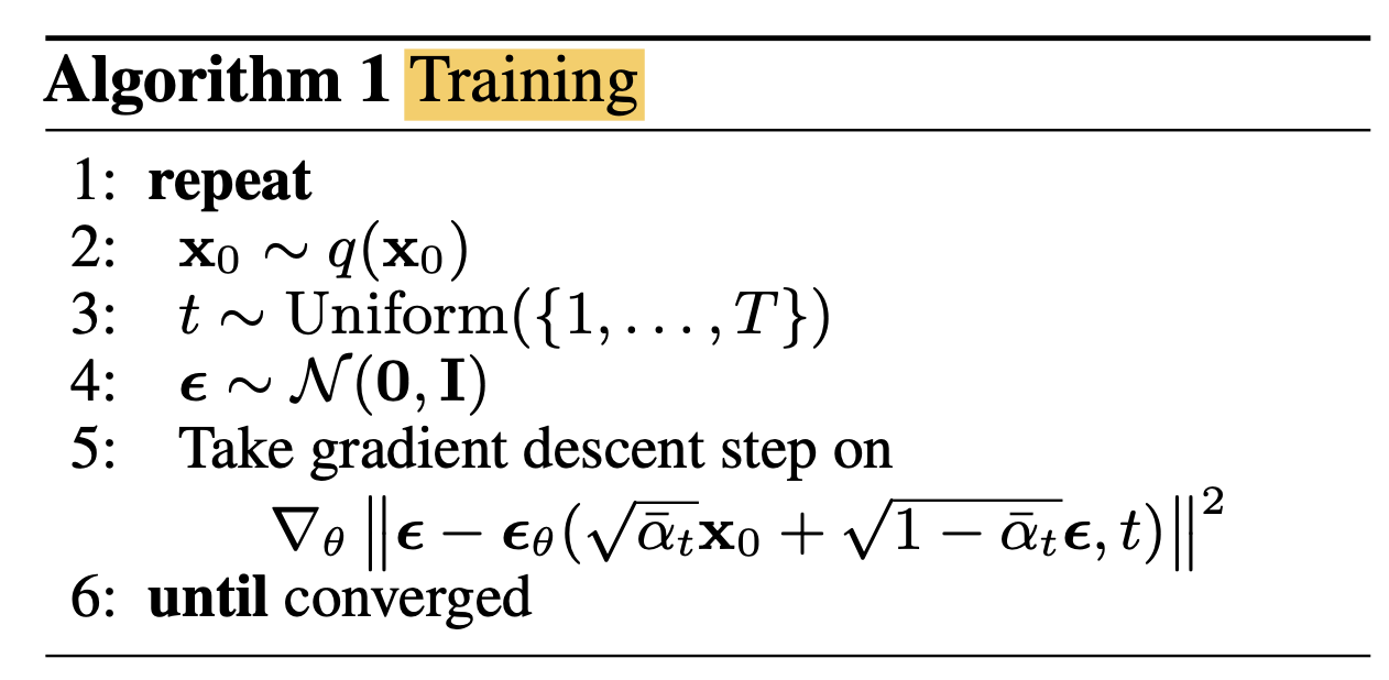Fig. Training Phase

여태 유도를 열심히 했으니 학습 과정은 아주 간단하게 이해할 수 있을겁니다.

• 데이터셋에서 배치 샘플링
• 데이터를 랜덤하게 더럽힌다. (t도 랜덤하게 정하고, \(\epsilon\)은 가우시안 분포에서 샘플링)
  • 이 과정에서 파라메터화 된 건 없음.
  • 더럽히는 과정은 반복적으로 할 필요가 없음. close form 으로 바로 더럽힐 수 있기 때문. ( \(\mathbf{x}_{t}\left(\mathbf{x}_{0}, \boldsymbol{\epsilon}\right)=\sqrt{\bar{\alpha}_{t}} \mathbf{x}_{0}+\sqrt{1-\bar{\alpha}_{t}} \boldsymbol{\epsilon} \text { for } \boldsymbol{\epsilon} \sim \mathcal{N}(\mathbf{0}, \mathbf{I})\) )
• Loss 를 계산하고 Gradient Descent
  • 당연히 Fully Differentiable 함 (reparam trick 을 썼기 때문에)
  • Loss Term은 아주 간단함. (\(\left[\left\|\boldsymbol{\epsilon}-\boldsymbol{\epsilon}_{\theta}\left(\sqrt{\bar{\alpha}_{t}} \mathbf{x}_{0}+\sqrt{1-\bar{\alpha}_{t}} \boldsymbol{\epsilon}, t\right)\right\|^{2}\right]\))

Inference Algorithm

추론 시에도 볼까요?

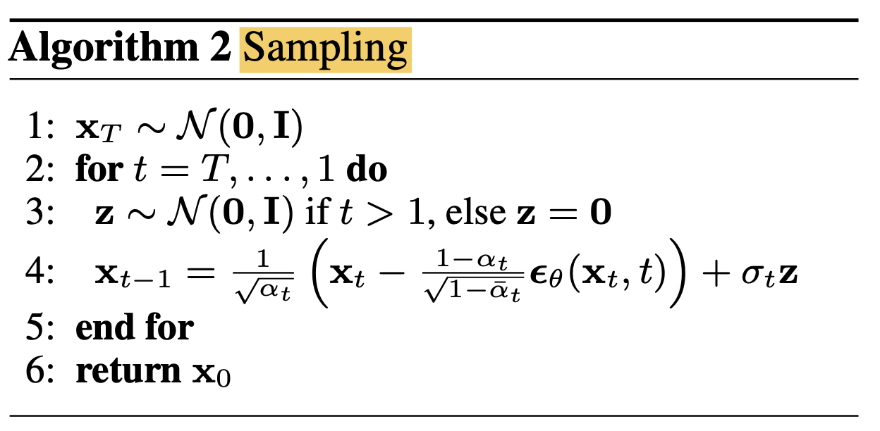Fig. Inferecne Phase

• 가우시안 노이즈를 뽑습니다. (T번 더럽혀진 상태라고 생각)
• T번 반복하면서 (\(x_{t-1} = \frac{ 1 }{ \sqrt{\sigma_t} } (x_t - \frac{ \beta_t }{ \sqrt{1-\bar{\sigma_t}} } \epsilon_{\theta} (x_t,t) ) + \sigma_t z\)) 수식으로 간단하게 이미지를 서서히 복원해 갑니다.
  • 기본적으로 \(\beta_t\) 는 상수
  • \[\alpha_t = 1-\beta_t\]
  • \[\bar{\alpha_t} = \Pi_{s=1}^t(\alpha_s)\]
  • \[\sigma^2_t = \beta^2\]

Model Architecture

Fig.

Results

실제 noise 로부터 Reverse Process를 통해 이미지를 복원하는 과정을 살펴봅시다.

첫 번째는 어떤 random bits 를 생성해서 반복적인 역과정을 통해 이미지를 복원한 케이스인데요,

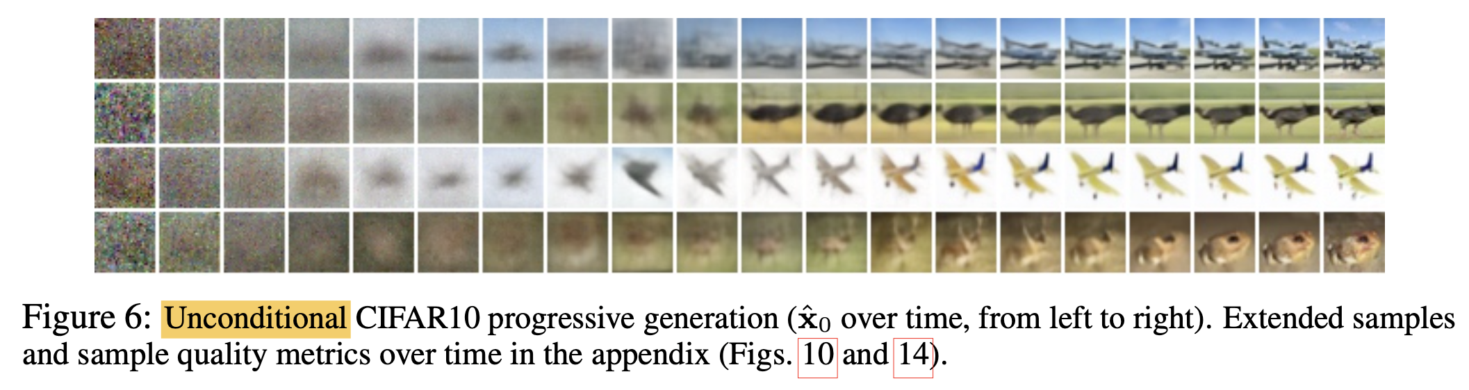
왼쪽부터 이미지가 \(T,T-1,\cdots,1,0\) 순서이며 점차 High Quality의 이미지가 만들어지는걸 알 수 있습니다.

그 다음으로는 \(\mathbf{x}_{0} \sim p_{\theta}\left(\mathbf{x}_{0} \mid \mathbf{x}_{t}\right)\), 즉 t번째 분포로부터 stochastic predictions을 한 결과입니다.

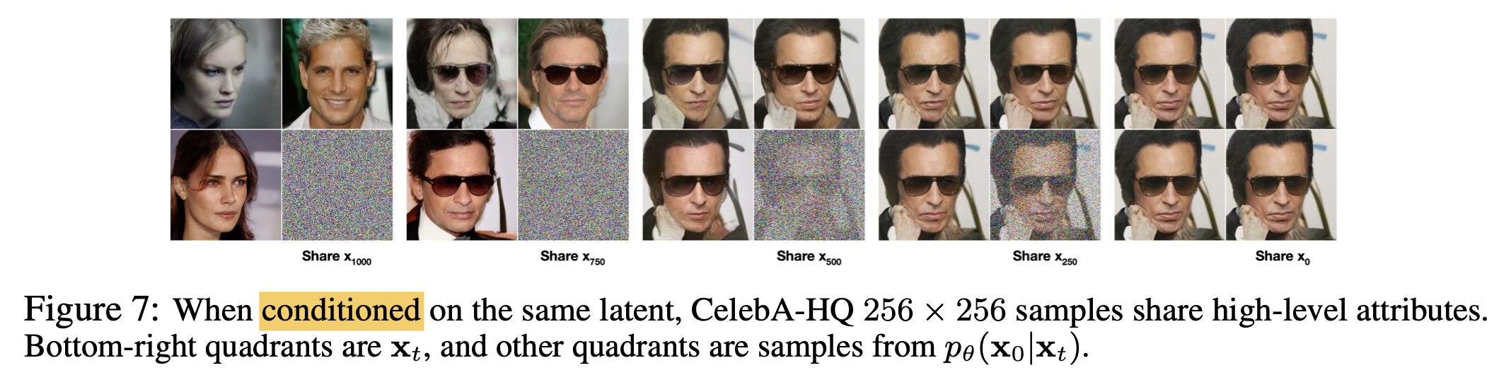
이미지에서 볼 수 있듯 t 값이 커질수록 큼지막한 feature들만 공유되고 (즉 이미지가 다양하게 생성됨), t 값이 작을수록 detail feature 들이 보존돼서 생성되는 이미지의 다양성이 줄어드는 걸 알 수 있습니다.

또한 생성 모델에서 빼놓을 수 없는 (?) Embedding Space 에서의 feature 들을 Interpolation 해보는 실험도 있는데요,

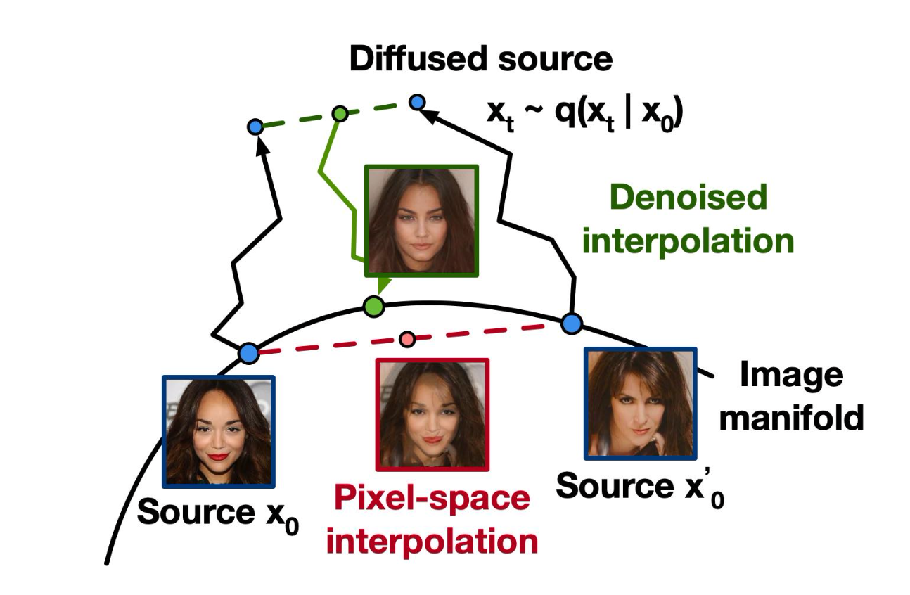Fig.

VAE 와 다르게 DDPM 에서는 인코더를 학습한 적이 없기 때죠. DDPM 에서 인코딩은 단순히 원본 이미지에 노이즈를 stochastic 하게 넣는것이기 때문에 준비한 이미지 2장에 각각 노이즈를 섞어준 뒤에

이를 디노이징 하면

두 원본 이미지의 feature 를 잘 반영한 결과를 얻을 수 있습니다.

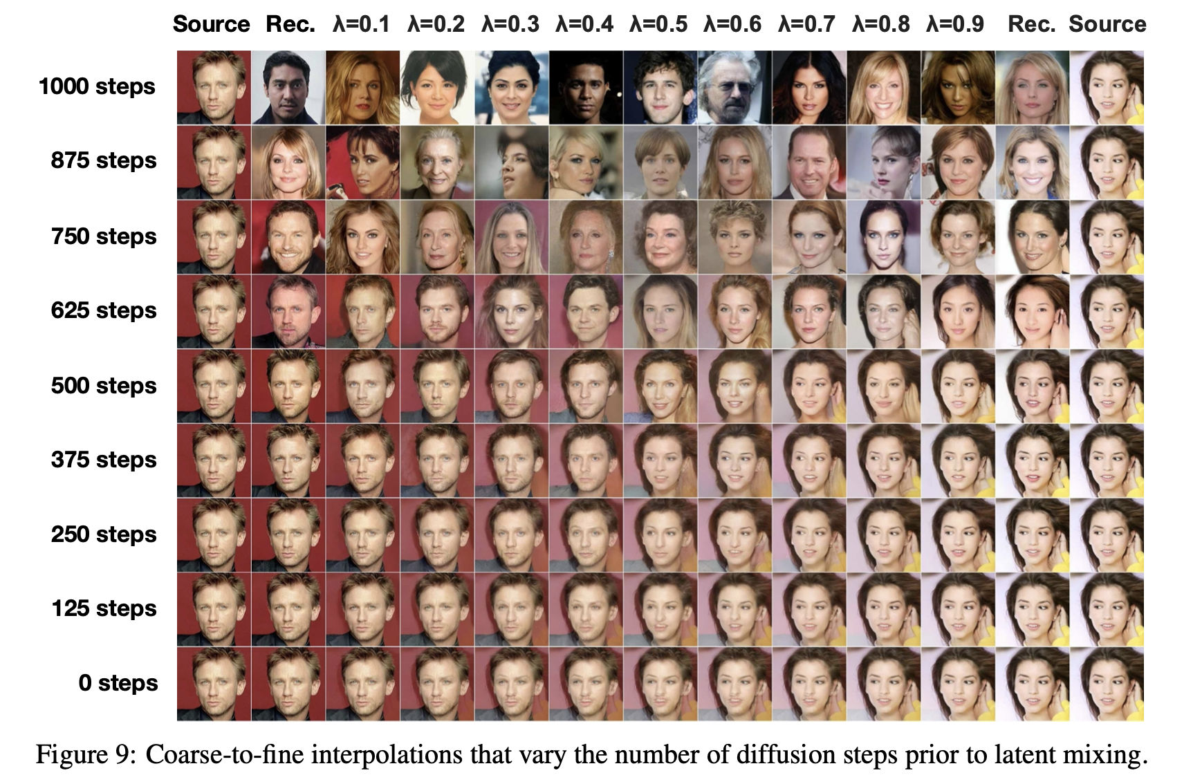Fig.

tmp

아래의 수식을

잘 변형하면 또 다른 form의 Objective를 유도할 수 있는데요,

References

• Papers
  • DALL-E
    • (DALL-E) Zero-Shot Text-to-Image Generation
    • (DALL-E 2) Hierarchical Text-Conditional Image Generation with CLIP Latents
  • Deep Unsupervised Learning using Nonequilibrium Thermodynamics
  • Denoising Diffusion Probabilistic Models
  • Denoising Diffusion Implicit Models
  • (CLIP) Learning Transferable Visual Models From Natural Language Supervision
  • Diffusion Models Beat GANs on Image Synthesis

  • GLIDE, Towards Photorealistic Image Generation and Editing with Text-Guided Diffusion Models

  • Understanding Diffusion Objectives as the ELBO with Simple Data Augmentation
• Github (Codes)
  • openai/DALL-E
  • openai/CLIP
  • openai/glide-text2im
  • glide-text2im/notebooks/inpaint.ipynb
  • lucidrains/DALLE-pytorch
  • karpathy/minGPT
  • kakaobrain/minDALL-E
  • Denoising Diffusion Probabilistic Models (DDPM) from labml.ai
  • DALL·E 2 Preview - Risks and Limitations
• Others (and Blogs)
  • https://drive.google.com/file/d/1p_aZ627Bwvku7nKyYRHtfZe50nAnpqGU/view
  • Diffusion Models as a kind of VAE from Angus Turner
  • What are Diffusion Models? from lillian weng
  • Generative Modeling by Estimating Gradients of the Data Distribution from Yang Song
  • (OpenAI Blog) CLIP: Connecting Text and Images
  • (OpenAI Blog) DALL·E: Creating Images from Text
  • (OpenAI Blog) DALL·E 2
  • Understanding VQ-VAE (DALL-E Explained Pt. 1)
  • How is it so good ? (DALL-E Explained Pt. 2)
  • DALL-E 2 vs Disco Diffusion
  • Introduction to Diffusion Models for Machine Learning from AssemblyAI
  • How DALL-E 2 Actually Works from AssemblyAI
  • How diffusion models work: the math from scratch (AI summer School)
  • How DALL·E 2 Works

  • An introduction to Diffusion Probabilistic Models from Ayan Das

  • The geometry of diffusion guidance
  • Building Diffusion Model’s theory from ground up from ICLR 2024 blog track